I’m currently working on the excellent Machine Learning course by Andrew Ng available on coursera. I’ve been working through the exercises using R, not matlab or octave as is requried in the course. This is the first programming exercise - implementing linear regression using the gradient descent algorithm rather than the normal equation method.
Gradient descent for a function with one parameter
Rather than calculating the optimal solution for the linear regression with a single algorithm, in this exercise we use gradient descent to iteratively find a solution. To get the concept behing gradient descent, I start by implementing gradient descent for a function which takes just on parameter (rather than two - like linear regression).
In this instance I have adapted code from Matt Bogard’s excellent blog Econometric Sense, and will use the same same function:
So we can state our objective to minimise $\theta_1$ with respect of $J(\theta_1)$ with a real number, or put mathetically $\min\limits_{\theta_1}J(\theta_1)$ and $\theta_1\in\mathbb{R}$
Cost function
We define the cost function $J(\theta_1)$ using calculus as $J(\theta)=2.4(x-2)$ (see Matt’s blog).
Gradient descent is defined by Andrew Ng as:
- where $\alpha$ is the learning rate governing the size of the step take with each iteration.
Here I define a function to plot the results of gradient descent graphically so we can get a sense of what is happening.
library(dplyr)
library(magrittr)
library(ggplot2)


xs <- seq(0,4,len = 100) # create some values

# define the function we want to optimize

f <-  function(x) {
  1.2 * (x-2)^2 + 3.2
  }

# plot the function

create_plot <- function(title) {
  plot(
    ylim = c(3,8),
    x = xs,
    y = f(xs),
    type = "l",
    ylab = expression(1.2(x-2)^2 + 3.2),
    xlab = "x",
    main = title
    )

  abline(
    h = 3.2,
    v = 2,
    col = "red",
    type = 2
    )

}

# J(theta)

cost <- function(x){
  1.2 * 2 * (x-2)
}
Below is the actual implementation of gradient descent.
# gradient descent implementation

grad <- function(x = 0.1, alpha = 0.6, j = 1000) {

  xtrace <- x
  ftrace <- f(x)

  for (i in 1:j) {

    x <- x - alpha * cost(x)

    xtrace <- c(xtrace,x)
    ftrace <- c(ftrace,f(x))

    }

  data.frame(
    "x" = xtrace,
    "f_x" = ftrace
    )
  }
Pretty simple! Now I use the plotting function to produce plots, and populate these with points using the gradient descent algorithm.
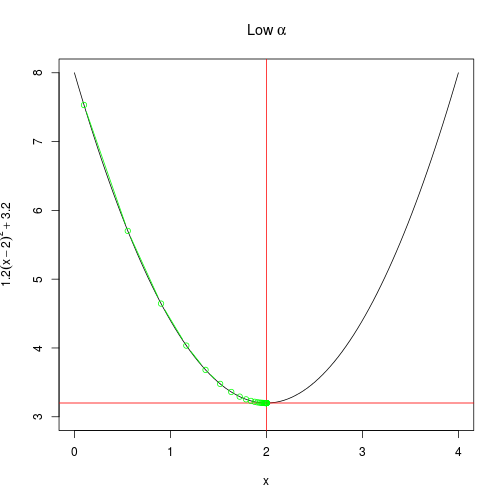
create_plot(expression(Low~alpha))

with(
  alpha_too_low <- grad(
    x = 0.1, # initialisation of x
    alpha = 0.1, # learning rate
    j = 100 # iterations
    ),
  points(
    x,
    f_x,
    type = "b",
    col = "green"
    )
  )
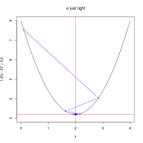
create_plot(expression(alpha~just~right))

with(
  alpha_just_right <- grad(
    x = 0.1, # initialisation of x
    alpha = 0.6, # learning rate
    j = 100 # iterations
    ),
  points(
    x,
    f_x,
    type = "b",
    col = "blue"
    )
  )
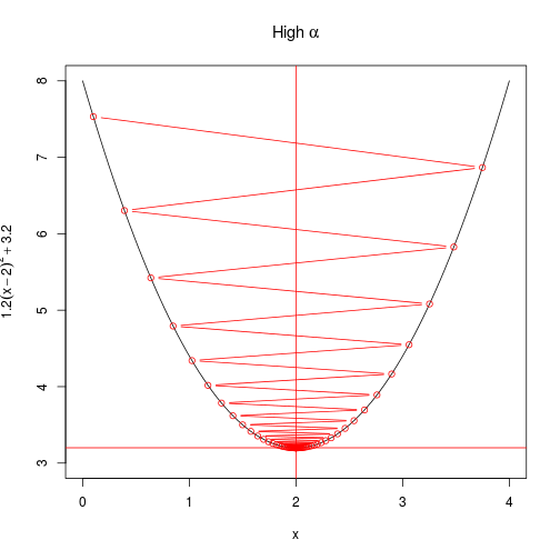
create_plot(expression(High~alpha))

with(
  alpha_too_high <- grad(
    x = 0.1, # initialisation of x
    alpha = 0.8, # learning rate
    j = 100 # iterations
    ),
  points(
    x,
    f_x,
    type = "b",
    col = "red"
    )
  )
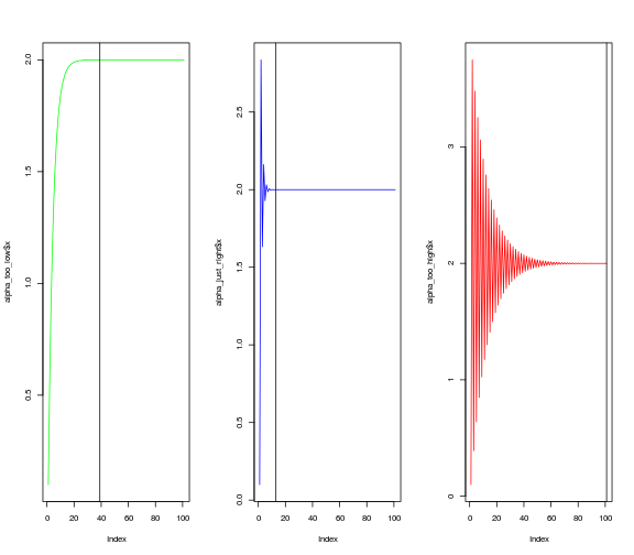
Another way to look at the rate of convergence is to plot the number of iterations against the output of $f(x)$. Vertical lines show when convergence occurs. When $\alpha$ is set very low, it takes much longer than necessary (although it does converge). When $\alpha$ is too high, convergence doesn’t occur at all within a hundred iterations.
par(mfrow=c(1,3))

plot(alpha_too_low$x, type = "l",col = "green")
abline(v = (round(alpha_too_low$x,4) != 2) %>% which %>% length)

plot(alpha_just_right$x, type = "l",col = "blue")
abline(v = (round(alpha_just_right$x,4) != 2) %>% which %>% length)

plot(alpha_too_high$x, type = "l", col = "red")
abline(v = (round(alpha_too_high$x,4) != 2) %>% which %>% length)