
I’ve been playing with implementations of linear and logistic regression over the last couple of months, following the exercises from a machine learning course that I have been doing. So far I have been writing things in a very functional way, constantly defining specific functions to do what are essentially generic things.
I’ve also started to write a couple of my own packages, one of which I have published on github and zenodo. This one provides access to an API which allows users to download data collected by GPS collars on cattle. This package is entirely written as functions.
So, I think that it is about time that I started to mature my R programming career, and start to write in classes. I’ve been following the excellent guide hosted on cran, by Friedrich Leisch, and in this post, I’m going to re-factor some of my previously functional code for linear regression with regularisation by implementing it with classes, and the usual model related methods like print(), summary(), and predict().
Before
So what does it look like at present? Rather than using the normal equation, this code uses the function optim to solve the problem:
optim takes in two functions, the cost function $J_\theta$ (J):
J <- function(X, y, theta, lambda) {

  m <- length(y)

  theta1 <- theta

  # Ensure that regularisation is not operating on \theta_0

  theta1[1] <- 0

  error <- tcrossprod(theta,X)
  error <- as.vector(error) - y
  error1 <- crossprod(error,error)

  reg <- (lambda/(2*m)) * crossprod(theta1, theta1)

  cost <- (1/(2 * m)) * error1 + reg

  return(cost)

}
and a gradient function (gR):
gR <- function(X, y, theta, lambda) {

  theta1 <- theta
  theta1[1] <- 0

  m <- length(y)

  error <- tcrossprod(theta,X)
  error <- as.vector(error) - y
  error <- (1/m) * crossprod(error,X)

  reg <- (lambda/(m)) * theta1

  delta <- error + reg

  return(delta)

}
These are taken as inputs in to the optim function:
theta <- rep(1,2)
lambda <- 0
x <- mpg$displ
y <- mpg$hwy

optim_out <- optim(
  par = theta,
  fn = function(t) J(cbind(1, x), y, t, lambda),
  gr = function(t) gR(cbind(1, x), y, t, lambda),
  method = "BFGS"
)
And calling this, we get:
optim_out## $par
## [1] 35.697650 -3.530589
##
## $value
## [1] 7.294506
##
## $counts
## function gradient
## 21 13
##
## $convergence
## [1] 0
##
## $message
## NULLJust to check, I compare this with a simple linear regression with lm().
lm_model <- lm(hwy ~ displ, data = mpg)
coef(lm_model)
## (Intercept) displ
## 35.697651 -3.530589So the coefficients are not the same, but are pretty close nonetheless.
all.equal(
  as.numeric(optim_out$par),
  as.numeric(coef(lm_model))
)
## [1] "Mean relative difference: 3.402685e-08"Converting to S3 classes and methods
Model function
As mentioned, I’m following this guide pretty closely, as it does exactly what I want to do. So I will start by producing a function to wrap up the optim call. optim must take inputs of functions for the cost and gradient, and so there is not too much that can be done to these functions as far as I can see, so for the moment I will leave them be.
vlrr_est <- function(x, y, lambda)

{

  theta <- rep(1,ncol(x))

  optim_out <- optim(
    par = theta,
    fn = function(t) J(x, y, t, lambda),
    gr = function(t) gR(x, y, t, lambda),
    method = "BFGS"
  )

  df = nrow(x) - ncol(x)

  # Calculate the variance

  sigma2 <- sum((y - x %*% optim_out$par)^2) / df

  # Compute covariance with sigma^2 * (X^{T}X)^-1. Note that Leisch counsels
  # against using this method of calculating the covariance matrix. Instead he
  # recommends using QR decomposition. As my present implementation does not
  # solve the normal equation (X^{T}X)^{−1}X^{T}y but instead relies on optim I
  # do not have the products of the QR decomposition to use in the matrix
  # inverse in the standard lm implementation: vcov <- sigma2 * chol2inv(qx$qr).
  # This implementation will do for now... Note that this requires MASS::ginv().
  # Mildly faster to use crossprod than %*%

  vcov <- sigma2 * ginv(crossprod(x,x))

  # Create a standardised output similar to that of lm()

  list(
    coefficients = optim_out$par,
    error = optim_out$value,
    convergence = optim_out$convergence,
    message = optim_out$message,
    vcov = vcov,
    sigma = sqrt(sigma2),
    df = df
    )
}
For now, x must be specified as the usual $\mathbb{R}^{m \times n+1}$ matrix consisting of a column of 1s which correspond to the intercept.
vlrr_est(x = cbind(1,mpg$displ), y = mpg$hwy, lambda = 0)## $coefficients
## [1] 35.697650 -3.530589
##
## $error
## [1] 7.294506
##
## $convergence
## [1] 0
##
## $message
## NULL
##
## $vcov
## [,1] [,2]
## [1,] 0.5189295 -0.13135737
## [2,] -0.1313574 0.03783558
##
## $sigma
## [1] 3.835985
##
## $df
## [1] 232So far so good. Now define the function vlrr() and the default method for it:
vlrr class and default method
# This is almost entirely lifted from Leisch (2009)

vlrr <- function(x, y, lambda, ...) UseMethod("vlrr")

vlrr.default <- function(x, y, lambda = 0, ...) {

  # Could put in some more verbose checks of the input here.

  x <- as.matrix(x)
  y <- as.numeric(y)
  lambda <- as.numeric(lambda)

  est <- vlrr_est(x, y, lambda)

  est$lambda = lambda
  est$fitted.values <- as.vector(x %*% est$coefficients)
  est$residuals <- y - est$fitted.values
  est$call <- match.call()

  class(est) <- "vlrr"
  est
}
So now if I call call vlrr or the vlrr.default function, I should get the same right?
identical(
  vlrr.default(cbind(1, mpg$disp), mpg$hwy, 0),
  vlrr(cbind(1, mpg$disp), mpg$hwy, 0)
)
## [1] TRUEAnd because I defined the output in a standard way, I can use the standard methods to interrogate it:
model <- vlrr(cbind(1, mpg$disp), mpg$hwy, 0)

coef(model)
## [1] 35.697650 -3.530589fitted.values(model) %>% head## [1] 29.34259 29.34259 28.63647 28.63647 25.81200 25.81200resid(model) %>% head## [1] -0.3425906 -0.3425906 2.3635271 1.3635271 0.1879979 0.1879979Print method
I won’t print(model) as at present is will print all the slots in turn:
attributes(model)## $names
## [1] "coefficients" "error" "convergence" "message"
## [5] "vcov" "sigma" "df" "lambda"
## [9] "fitted.values" "residuals" "call"
##
## $class
## [1] "vlrr"This ends up being very long, so it would be good to write a print method that returns something a bit shorter.
print.vlrr <- function(x, ...) {
  cat("Call:\n")
  print(x$call)
  cat("\nError:\n")
  print(x$error)
  cat("\nCoefficients:\n")
  print(x$coefficients)
}

print(model)
## Call:
## vlrr.default(x = cbind(1, mpg$disp), y = mpg$hwy, lambda = 0)
##
## Error:
## [1] 7.294506
##
## Coefficients:
## [1] 35.697650 -3.530589Better.
Summary method
Model functions also usually have a summary method which prints out a nice summary of the model (e.g. summary.lm). For now I’ll just copy the default method given by Leisch, plus additional information about optim’s convergence success.
summary.vlrr <- function(object, ...) {


  # It would be nice to be able to compare the success of models from the
  # summary output. Here I include a simple mean squared error.

  m <- length(object$fitted.values)
  error <- object$residuals
  MSE <- as.numeric(1/m * crossprod(error, error))

  se <- sqrt(diag(object$vcov))
  tval <- coef(object) / se

  # Note that here the p value is for testing the null hypothesis that the
  # coefficients are different from zero


  TAB <- cbind(
    Estimate = coef(object),
    StdErr = se,
    t.value = tval,
    p.value = 2*pt(-abs(tval), df=object$df)
  )
  res <- list(
    convergence = object$convergence,
    message = object$message,
    call = object$call,
    coefficients = TAB,
    MSE = MSE
  )

  class(res) <-"summary.vlrr"
  res
}

summary(model)
## $convergence
## [1] 0
##
## $message
## NULL
##
## $call
## vlrr.default(x = cbind(1, mpg$disp), y = mpg$hwy, lambda = 0)
##
## $coefficients
## Estimate StdErr t.value p.value
## [1,] 35.697650 0.7203676 49.55477 2.123533e-125
## [2,] -3.530589 0.1945137 -18.15085 2.038996e-46
##
## $MSE
## [1] 14.58901
##
## attr(,"class")
## [1] "summary.vlrr"This is a bit messy, but we can define a print method for summary using the Coefmat function to order things nicely in the coefficients table.
print.summary.vlrr <- function(x, ...) {

  cat("Vectorised linear regression by optim:\n")
  cat("\n")
  cat("Convergence (see ?optim):\n")
  print(x$convergence)
  print(x$message)

  cat("\n")
  cat("Call:\n")

  print(x$call)
  cat("\n")

  cat("Lambda:\n")

  print(x$lambda)
  cat("\n")

  printCoefmat(
    x$coefficients,
    P.value = TRUE,
    has.Pvalue = TRUE
  )

  cat("\n")
  cat("MSE:\n")
  print(x$MSE)
}

print(summary(model))
## Vectorised linear regression by optim:
##
## Convergence (see ?optim):
## [1] 0
## NULL
##
## Call:
## vlrr.default(x = cbind(1, mpg$disp), y = mpg$hwy, lambda = 0)
##
## Lambda:
## NULL
##
## Estimate StdErr t.value p.value
## [1,] 35.69765 0.72037 49.555 < 2.2e-16 ***
## [2,] -3.53059 0.19451 -18.151 < 2.2e-16 ***
## ---
## Signif. codes: 0 '***' 0.001 '**' 0.01 '*' 0.05 '.' 0.1 ' ' 1
##
## MSE:
## [1] 14.58901Great, so this looks a lot more like the output we would expect from lm(), plus we have some statistics on the likelihood that our coefficients are different from zero.
Formula method
It’s a bit tiresome having to specify x= and y= when in lm() and other models, we are able to specify a formula. In addition, if we want to include interaction terms $x_1 \times x_2$ for instance, this would need to be done in the input matrix x. By implementing a formula method, this can all be automated. This also gets us off the hook with having to cbind(1,x).
At present I must do:
vlrr(x=cbind(1,x),y=y)But after implementing the formula method…
vlrr.formula <- function(formula, data = list(), ...) {

  mf <- model.frame(formula = formula, data = data)
  x <- model.matrix(attr(mf, "terms"), data = mf)
  y <- model.response(mf)

  est <- vlrr.default(x, y, ...)
  est$call <- match.call()
  est$formula <- formula
  est

}
…things get much much simpler!
model <- vlrr(hwy ~ displ,lambda = 0, data = mpg)
print(model)
## Call:
## vlrr.formula(formula = hwy ~ displ, data = mpg, lambda = 0)
##
## Error:
## [1] 7.294506
##
## Coefficients:
## [1] 35.697650 -3.530589and how about:
summary(model)## $convergence
## [1] 0
##
## $message
## NULL
##
## $call
## vlrr.formula(formula = hwy ~ displ, data = mpg, lambda = 0)
##
## $coefficients
## Estimate StdErr t.value p.value
## [1,] 35.697650 0.7203676 49.55477 2.123533e-125
## [2,] -3.530589 0.1945137 -18.15085 2.038996e-46
##
## $MSE
## [1] 14.58901
##
## attr(,"class")
## [1] "summary.vlrr"Predict method
The last method I want to implement is predict as this makes it much easier to use the model once fit. Again I’m relying on Leisch here.
predict.vlrr <- function(object, newdata = NULL, ...) {

  # If no new data, the just present the fitted values from the model

  if(is.null(newdata)) {
    y <- fitted(object)
  }
  else{
    if(!is.null(object$formula)){
      ## model has been fitted using formula interface
      x <- model.matrix(object$formula, newdata)
    }
    else{
      # newdata is just a matrix
      x <- newdata
    }
    y <- as.vector(x %*% coef(object))
  }
  y
}
Testing it out
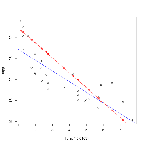
So finally we can take this model and apply it to some other data. Here I take the model I built on fuel consumption from the mpg dataset, and use it to predict displacement values (disp) from the mtcars dataset. Note that displacement is given in cubic inches in mtcars but litres in mpg so needs to be multiplied by 0.0163 to put it on the same scale.
# Create base plot and fit using lm

plot(
  mpg ~ I(disp * 0.0163),
  data = mtcars,
  title = "mtcars"
)

abline(
  lm(mpg~I(disp * 0.0163), data = mtcars),
  col = "blue",
  type = "o"
  )

# Use predict method on mpg model and predict over new data

new_y <- predict(
  model,
  newdata = list(hwy = mtcars$disp, displ = mtcars$disp * 0.0163)
)

points(
  mtcars$disp * 0.0163,
  new_y,
  col = "red",
  type = "o"
)
Writing a package
So the obvious thing to do now that this has all been done, is to wrap everything up into a package. I’m not going to go through the steps to do that here because it is a little bit long winded, and much better covered in the Leisch guide, and here by Hadley Wickham.
It’s a pretty simple process, and actually the most onerous (and arguably the most important) thing is to properly document all the functions. So I have put in a little bit of time, and produced the package vlrr, which is now available from a github repo.
This can be installed direct from within R using devtools::install_github("ivyleavedtoadflax/vlrr"). The library can then be called and run like any other.
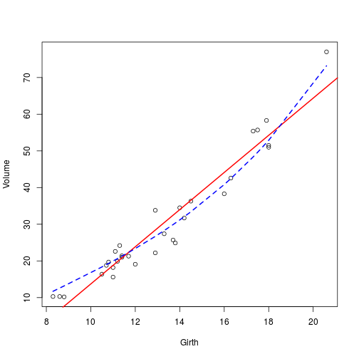
library(vlrr)

model <- vlrr(Volume ~ Girth, data = trees)

summary(model)
## Vectorised linear regression by optim:
##
## Convergence (see ?optim):
## [1] 0
## NULL
##
## Call:
## vlrr.formula(formula = Volume ~ Girth, data = trees)
##
## Lambda:
## NULL
##
## Estimate StdErr t.value p.value
## [1,] -36.94331 3.36514 -10.978 7.622e-12 ***
## [2,] 5.06585 0.24738 20.478 < 2.2e-16 ***
## ---
## Signif. codes: 0 '***' 0.001 '**' 0.01 '*' 0.05 '.' 0.1 ' ' 1
##
## MSE:
## [1] 16.91299plot(Volume ~ Girth,data = trees)
abline(
model,
col = "red",
lwd = 2
)
# Something more complicated
model1 <- vlrr(Volume~poly(Girth,degree = 3), lambda = 0.1,data = trees)
summary(model1)## Vectorised linear regression by optim:
##
## Convergence (see ?optim):
## [1] 0
## NULL
##
## Call:
## vlrr.formula(formula = Volume ~ poly(Girth, degree = 3), data = trees,
## lambda = 0.1)
##
## Lambda:
## NULL
##
## Estimate StdErr t.value p.value
## [1,] 30.17097 0.66188 45.5839 < 2.2e-16 ***
## [2,] 79.15766 3.68518 21.4800 < 2.2e-16 ***
## [3,] 13.26527 3.68518 3.5996 0.001263 **
## [4,] 2.75774 3.68518 0.7483 0.460729
## ---
## Signif. codes: 0 '***' 0.001 '**' 0.01 '*' 0.05 '.' 0.1 ' ' 1
##
## MSE:
## [1] 11.82823lines(
trees$Girth,
model1$fitted.values,
col = "blue",
lwd = 2,
lty = 2
)
sessionInfo() ## R version 3.2.0 (2015-04-16)
## Platform: x86_64-unknown-linux-gnu (64-bit)
## Running under: Ubuntu 14.04.2 LTS
##
## locale:
## [1] LC_CTYPE=en_GB.UTF-8 LC_NUMERIC=C
## [3] LC_TIME=en_GB.UTF-8 LC_COLLATE=en_GB.UTF-8
## [5] LC_MONETARY=en_GB.UTF-8 LC_MESSAGES=en_GB.UTF-8
## [7] LC_PAPER=en_GB.UTF-8 LC_NAME=C
## [9] LC_ADDRESS=C LC_TELEPHONE=C
## [11] LC_MEASUREMENT=en_GB.UTF-8 LC_IDENTIFICATION=C
##
## attached base packages:
## [1] methods stats graphics grDevices utils datasets base
##
## other attached packages:
## [1] vlrr_0.1 MASS_7.3-40 tidyr_0.2.0 ggplot2_1.0.1
## [5] ucminf_1.1-3 boot_1.3-16 magrittr_1.5 dplyr_0.4.1
## [9] testthat_0.9.1 knitr_1.10
##
## loaded via a namespace (and not attached):
## [1] Rcpp_0.11.5 munsell_0.4.2 colorspace_1.2-6
## [4] stringr_1.0.0 plyr_1.8.2 tools_3.2.0
## [7] parallel_3.2.0 grid_3.2.0 gtable_0.1.2
## [10] DBI_0.3.1 checkpoint_0.3.10 assertthat_0.1
## [13] digest_0.6.8 reshape2_1.4.1 formatR_1.2
## [16] evaluate_0.7 stringi_0.4-1 scales_0.2.4
## [19] proto_0.3-10