
I’ve been working on a chapter of a book looking at weather and production data for a major crop across the globe. One of the things I need to produce is a bubble map showing the relative production for each producing country worldwide, and region specific maps for each of the major production growing region.
There is a great package for doing this called rworldmap. In this little post I present the code I used to produce figures for the book using rworldmap.
Getting the data
First thing first, I need some data. The UN FAO very helpfully make these data available online, but it also turns out that there is an API and an R package to access that API called FAOSTAT.
The FAOSTAT package
The FAOSTAT package has a really simple interface that allows you to navigate through the available statistics, and download what you want. For example, I’m interested in the production and yield statistics for apple production within every apple producing region in the world
install.packages("FAOSTAT")
library(FAOSTAT)

# Create an object named '.LastSearch' using the FAOSearch function, which can then be called as an argument to the getFAO() or getFAOtoSYB() function.

FAOsearch()

# Now get the data

apple_data <- getFAOtoSYB(query = .LastSearch)
A slightly easier way of dealing with the information that comes back from the query is as follows:
apple_df <- data.frame(
  varName = c("areaHarvested", "yield", "extractionRate","production","seed"),
  domainCode = "QC",
  itemCode = 515,
  elementCode = c(5312,5419,5423,5510,5525),
  stringsAsFactors = FALSE
)

apple_df_lst <- with(
  apple_df,
  getFAOtoSYB(
    name = varName,
    domainCode = domainCode,
    itemCode = itemCode,
    elementCode = elementCode,
    useCHMT = TRUE,
    outputFormat = "long"
  )
)
Note that the useCHMT option will clean up the data somewhat, as FAO data can double count territories like China, because of Taiwan, and Hong Kong. This check can also be conducted manually outside of the getFAO function.
The FAOSTAT package includes a function translateCountryCode() which allows the UN numeric country code to be translated to an ISO2 or ISO3 letter code. In the current instance this is not a problem, because rworldwap will take numeric UN codes.
The rworldmap package
Next step is to tidy up the FAOSTAT data before it can joined to a country map in rworldmap. Initially, I am only interested in the most up-to-date production, so I’ll filter these out.
# Data from FAOSTAT 2013 apple yields

apple2013 <- apple_df_lst$entity %>%
  dplyr::filter(
    name == "production",
    Year == 2013
  )
Now try to join this data to a map.
library(rworldmap)

sPDF <- joinCountryData2Map(
  apple2013,
  joinCode = "UN",
  nameJoinColumn = "FAOST_CODE"
)
## 27 codes from your data successfully matched countries in the map
## 68 codes from your data failed to match with a country code in the map
## 217 codes from the map weren't represented in your dataSo there is a problem here; 68 of the codes in the apple2013 data failed to match up with data on the map. I’ll try to plot it anyway, and see what happens.
par(
  mai = c(0,0,0.2,0),
  xaxs = "i",
  yaxs = "i"
)

mapCountryData(
  sPDF,
  nameColumnToPlot="Value"
)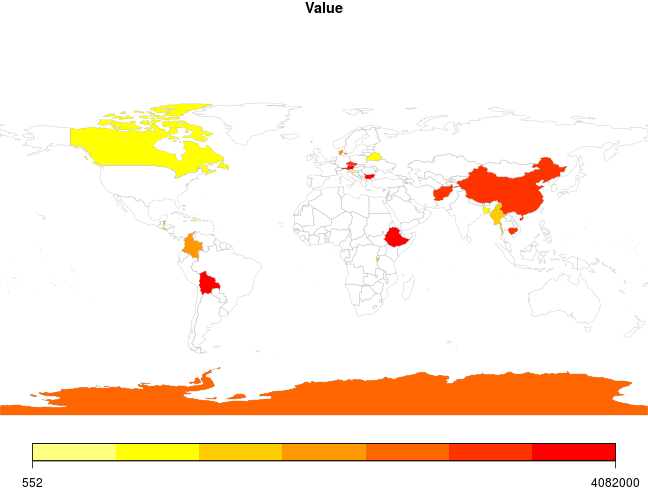
There’s definitely something funny going on here, because Antarctica is not known for its apple growing regions. Evidently there is more of a problem than was suggested in the mis-match warning.
I’ll try to solve this by converting the UN codes to ISO3 codes, although as noted in the FAOSTAT vignette there are some problems which are not addressed by the ISO coding system, for instance the change of names or lack of recognition (at the UN) of certain countries.
apple2013 <- translateCountryCode(
  data = apple2013,
  from = "FAOST_CODE",
  to = "ISO3_CODE"
)
##
## NOTE: Please make sure that the country are matched according to their definitionsPDF <- joinCountryData2Map(
apple2013,
joinCode = "ISO3",
nameJoinColumn = "ISO3_CODE",
verbose = TRUE
)## 94 codes from your data successfully matched countries in the map
## 1 codes from your data failed to match with a country code in the map
## failedCodes
## [1,] "REU"
## 150 codes from the map weren't represented in your dataBetter, but REU - Reunion island has not been matched probably because it has an accent over the e. It’s not critical for this demonstration, so I will leave it unmatched
Bubble maps
Adjusting the previous code to produce a bubble map is pretty simple. However producing legends in rworldmap does not yet allow much customisation. I found a hacky solution to get the look I wanted.
Firstly, I didn’t want the numbers in the legend to appear as exponents, so I set options("scipen" = 10) to allow these numbers to be displayed in full.
The next problem I ran into was that in the current version of rworldmap (1.3-1) I couldn’t find a way to synchronise the colour of the map bubbles with the legend bubbles, nor could I seem to get the legend bubbles to be filled. To get round this, I cheated a bit here, and downloaded, edited the file containing the mapBubbles function (mapBubbles.r), and hardcoded the legend symbols to be "red" and pch = 19, to match the map itself. I also added an option to the legend call in mapBubbles() so that by default the colour of the border matches the border background. At present these changes are hardcoded as I need a quick fix, but if I get a chance I will make better implementations and submit them as pull requests to the github repo. For now, I unzipped the package to a folder, made my changes then called devtools::load_all() to load the altered package (I would have re-packaged it, but ran int some errors which I did not have the patience to fix).
options("scipen" = 10)

par(
  mai = c(0, 0, 0.2, 0),
  xaxs = "i",
  yaxs = "i"
)

mapBubbles(
  dF = sPDF,
  nameZSize="Value",
  #nameZColour="Value",
  oceanCol = "white",
  landCol = "gray90",
  borderCol = "black",
  addLegend = TRUE,
  legendVals = c(10000,100000,1000000,25000000),
  legendTitle = expression(Tonnes~yr^-1),
  legendBg = "white",
  legendPos = "left",
  addColourLegend = TRUE
)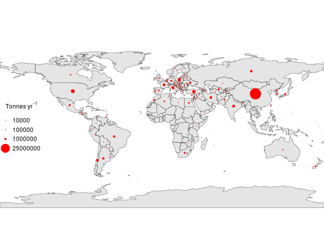
So after all that, this is what I get. A bit more complicated than using a point and click GIS for pretty similar results, and a bit of a quick fix. If I need to make more of these kinds of visualisation, there are some really beautiful ways of doing this with D3.js; this (or this) is probably how I would do it next time.
sessionInfo()## R version 3.2.2 (2015-08-14)
## Platform: x86_64-pc-linux-gnu (64-bit)
## Running under: Ubuntu 14.04.3 LTS
##
## locale:
## [1] LC_CTYPE=en_GB.UTF-8 LC_NUMERIC=C
## [3] LC_TIME=en_GB.UTF-8 LC_COLLATE=en_GB.UTF-8
## [5] LC_MONETARY=en_GB.UTF-8 LC_MESSAGES=en_GB.UTF-8
## [7] LC_PAPER=en_GB.UTF-8 LC_NAME=C
## [9] LC_ADDRESS=C LC_TELEPHONE=C
## [11] LC_MEASUREMENT=en_GB.UTF-8 LC_IDENTIFICATION=C
##
## attached base packages:
## [1] methods stats graphics grDevices utils datasets base
##
## other attached packages:
## [1] rworldmap_1.3-1 FAOSTAT_2.0 ggmap_2.4 ggplot2_1.0.1
## [5] sp_1.1-1 readr_0.1.1 magrittr_1.5 dplyr_0.4.2
## [9] testthat_0.9.1 knitr_1.11
##
## loaded via a namespace (and not attached):
## [1] Rcpp_0.12.0 git2r_0.10.1 formatR_1.0
## [4] plyr_1.8.3 class_7.3-13 tools_3.2.2
## [7] digest_0.6.8 memoise_0.2.1 evaluate_0.7.2
## [10] gtable_0.1.2 lattice_0.20-33 png_0.1-7
## [13] DBI_0.3.1 mapproj_1.2-3 curl_0.9.1
## [16] parallel_3.2.2 spam_1.0-1 proto_0.3-10
## [19] e1071_1.6-6 roxygen2_4.1.1 xml2_0.1.1
## [22] stringr_0.6.2 rversions_1.0.2 devtools_1.8.0
## [25] RgoogleMaps_1.2.0.7 fields_8.2-1 maps_2.3-10
## [28] classInt_0.1-22 grid_3.2.2 data.table_1.9.4
## [31] R6_2.1.0 jpeg_0.1-8 foreign_0.8-65
## [34] RJSONIO_1.3-0 reshape2_1.4.1 scales_0.2.5
## [37] maptools_0.8-36 MASS_7.3-43 assertthat_0.1
## [40] checkpoint_0.3.10 colorspace_1.2-6 geosphere_1.4-3
## [43] labeling_0.3 lazyeval_0.1.10 munsell_0.4.2
## [46] chron_2.3-47 rjson_0.2.15