
A more formalised implementation of regularisation
A short while ago I published a post based on an exercise from Andrew Ng’s Machine Learning course on Coursera. In that post I implemented regularisation for a vectorised implementation of linear regression. In reality when approaching a machine learning problem, I wouldn’t want to rely on functions I have written myself when there are fully formed packages supporting these techniques. So in this post I’m going to reproduce the analysis from my previous post but using the R package glmnet. Glmnet is a package of functions for generalised linear models that has been implement in R by Trevor Hastie and Junyang Qian.
In my previous post, the code I implemented solved the minimisation problem:
where the first summation is essentially the usual sum of the squared differences between the expected and the observed, and the addition is the regularisation term.
The glmnet function solves the problem1:
There are a few additional parameters here, but fundamentally the problem is the same. The function $l(y,\eta)$ for the Gaussian case (i.e. a simple linear model with a normal error structure) is equivalent to $\frac{1}{2}(y-\eta)^2$,and we can make the regularisation term look a lot more familiar by referring to Friedman et al. (2010)2.
So this is much closer to the problem I was working with before. $\vec{w}$ is simply a vector of weights of length $m$ which default to 1. Then there is the parameter $\alpha$ which controls the rather enigmatically named elastic-net penalty ($a\in{0,1}$). We see the original summation of the $j$ elements of $\theta$ ($\sum^n_{j=1} \theta^{2}_j$), but each element is multiplied by $\frac{1}{2}(1-\alpha)$ (also $(1-a)\in{0,1}$) to which $\alpha \times$ the absolute value of $\theta_j$ is added.
$\alpha$ is important: setting $\alpha = 1$ will result in lasso regularisation, whilst $\alpha = 0$ gives you ridge regularisation. The practical significance of this is that using ridge regression will not totally remove features from the regression, but just reduces their importance. Lasso on the other hand will set parameters to zero, thus removing features from the regression3 entirely. $\alpha$ is thus set somewhere between the two extremes; according to the documentation, setting $\alpha=0.5$ is effective in selecting groups of correlated features, and including or excluding them from the model.
So with a little digging, this equation is not quite as scary as it first looked, and is not so different from the regularisation that I have already been using.
glmnet in action
For this example, I again use the mtcars dataset, and make the same split of the data as before. So in the training set $m=19$ and $n = 3$: cyl, disp, hp.
Here’s what it looks like:
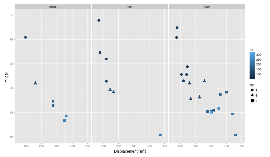
From here on I follow the quick start guide in the glmnet documentation. To start with, I’ll stick to just the original features, and not add any polynomials as before.
y <- train$mpg

# Note that it is not necesary to include a column of ones as it was in my
# implementation. Actually it doesn't matter if you do, this just gets
# simplified away.

X_train <- cbind(train$cyl,train$disp,train$hp)
The simple use case is as follows:
fit = glmnet(X_train,y)When printed, this gives a summary of each step towards minimisation with the number of coefficients not set to zero (Df), the % of null deviance the model explains, and the value of $\lambda$ that was tried. In the present case, the process stops early at 55 (default is 100) because the deviance explained had remained fairly constant.
We can use the coef method to extract the coefficients for a given $\lambda$. Setting $\lambda=0$, i.e. no regularisation results in very similar coefficients returned in my previous post for the simple linear multiple regression.
coef(fit, s = 0)## 4 x 1 sparse Matrix of class "dgCMatrix"
## 1
## (Intercept) 30.18697602
## V1 -2.37918214
## V2 -0.01362517
## V3 -0.01428008And it looks pretty linear (in this and all the plots that follow, the red symbols are the values predicted by the model, whilst blue are the training/test set values):
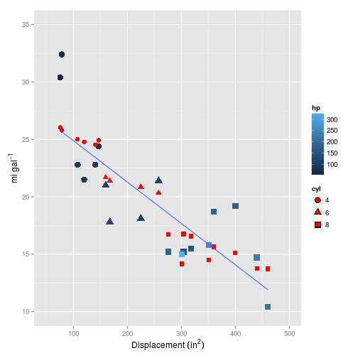
Note that if you don’t specify a $\lambda$ with s=0, then predict will return all the models evaluated - in this case 55.
To choose a model, we can use cross validation which is nicely implemented in the cv.glmnet() function, and specified in the same way. For this example I’m going to add third order polynomials to $X$ to try to capture some of the curvature evident in the plots.
X_train_3 <- poly(X_train, degree = 3, raw = TRUE)On $n=3$ features, this results in $n=19$ total features after creation of polynomials, on just $m=19$ training examples. So this model could lead to bad overfitting, but is a great chance to test out regularisation.
cvfit <- cv.glmnet(
  x = X_train_3,
  y = y
)
Again, printing this object will give a list of all the models tried, with varying $\lambda$, but with two additional slots: $lambda.min, and $lambda.1se. These are respectively the value of $\lambda$ that gives the minimum mean cross-validated error, and the value of $\lambda$ which gives the most heavily regularised model, but is still within 1 standard error of $lambda.min.
We can extract the coefficients for these with:
coef(cvfit,"lambda.min")## 20 x 1 sparse Matrix of class "dgCMatrix"
## 1
## (Intercept) 29.71516838
## 1.0.0 -2.33870568
## 2.0.0 .
## 3.0.0 .
## 0.1.0 -0.01290432
## 1.1.0 .
## 2.1.0 .
## 0.2.0 .
## 1.2.0 .
## 0.3.0 .
## 0.0.1 -0.01287220
## 1.0.1 .
## 2.0.1 .
## 0.1.1 .
## 1.1.1 .
## 0.2.1 .
## 0.0.2 .
## 1.0.2 .
## 0.1.2 .
## 0.0.3 .Note that a full stop would indicate that the parameter have been set to zero. Interestingly, after cross-validation only the original features have been retained. A plot of the object cv.fit is informative, and shows that the best mean squared errors are obtained with only three parameters.
plot(cvfit)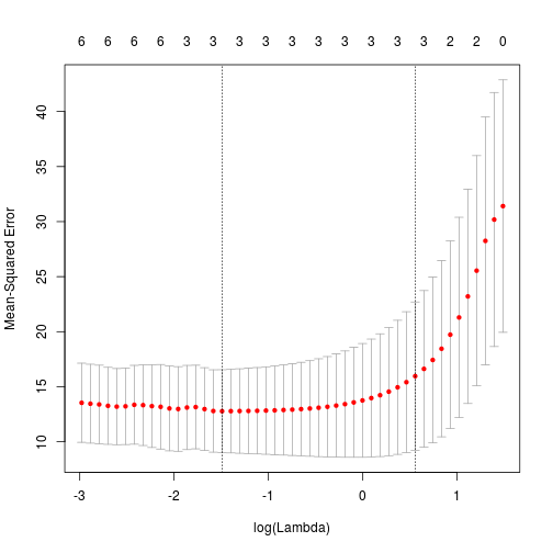
This may suggest that to retain more parameters in the model, I need to adjust the $\alpha$ parameter closer to 0, (i.e. ridge regression) which will not remove parameters from the model totally.
Comparing the result here (using the $J_{train}$ function I defined previously with the training errors obtained in the previous post, neither of the two models (lambda.min and lambda.1se) match the performance of the regularised models which retained all 19 parameters ($\approx 4$).
J_train(
  predicted = predict(cvfit, newx = X_train_3,s = "lambda.min"),
  actual = train$mpg
) %>%
  round(2)
## 1
## 1 7.95So let’s try again, this time adjusting the parameter $\alpha$.
cvfit_a0 <- cv.glmnet(
  x = X_train_3,
  y = y,
  alpha = 0
)

coef(cvfit_a0,s="lambda.min")
## 20 x 1 sparse Matrix of class "dgCMatrix"
## 1
## (Intercept) 2.344421e+01
## 1.0.0 -2.337616e-01
## 2.0.0 -5.381901e-02
## 3.0.0 -1.512854e-02
## 0.1.0 -1.594568e-03
## 1.1.0 -3.903502e-04
## 2.1.0 -1.119476e-04
## 0.2.0 -2.487628e-06
## 1.2.0 -7.425475e-07
## 0.3.0 -4.680394e-09
## 0.0.1 -2.219181e-03
## 1.0.1 -5.714757e-04
## 2.0.1 -1.656194e-04
## 0.1.1 -4.479784e-06
## 1.1.1 -1.309593e-06
## 0.2.1 -9.248751e-09
## 0.0.2 -4.111644e-06
## 1.0.2 -1.276034e-06
## 0.1.2 -1.175934e-08
## 0.0.3 -8.464555e-09OK so this time we have retained all of the parameters, but the coefficients are very small, and unlikely to wield much influence on the model.
So what about the errors? the $\alpha=0$ ridge model fares less well than the $\alpha=0.5$ elastic-net model.
##      1
## 1 12.7
Of course this is training set error. What about the test set?
## 1
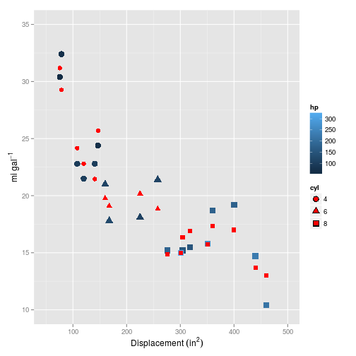
## 1 5.33How does this look plotted? First $\alpha=0.5$ (the default):
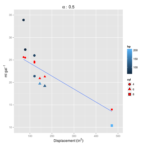
And for $\alpha = 0$.
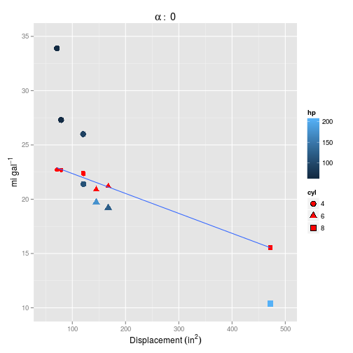
Setting $\alpha=0$ definitely makes things worse, but neither model captures the curvature inherent in the data.
A simpler model
OK so $m=n$ is a pretty extreme example which is a bit out of the ordinary. I’ll repeat the above with only using a second degree polynomial which gives $n=9$ features.
X_train_2 <- poly(X_train, degree = 2, raw = TRUE)

cvfit_2 <- cv.glmnet(
  x = X_train_2,
  y = y
)

coef(cvfit_2,s="lambda.min")
## 10 x 1 sparse Matrix of class "dgCMatrix"
## 1
## (Intercept) 45.0055788920
## 1.0.0 2.5275893500
## 2.0.0 -9.5882447634
## 0.1.0 -0.0974340343
## 1.1.0 0.1195261643
## 0.2.0 -0.0003053265
## 0.0.1 -0.1975309143
## 1.0.1 0.0851493804
## 0.1.1 -0.0002147503
## 0.0.2 .With just second degree polynomials and the default $\alpha = 0.5$, most of the parameters have been retained in the model, and the error is looking a lot smaller:
##      1
## 1 2.61
But how does it plot?
Now this is looking much more promising! How does it fare on the test set?
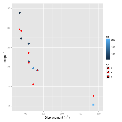
Also looking like a pretty strong fit. And the error?
##      1
## 1 2.59
Interestingly this is slightly higher than the errors of 1.00 and 1.03 achieved in using the simpler code I implemented in my earlier post. This is surprising, as intuitively from plots I would have said that the glmnet model has performed better. I may have to check this…
It’s also interesting to see that glmnet did not perform well when I included the extreme case scenario of a single feature for a single training example, yet the simpler algorithm I implemented produced almost identical results when including second or third order polynomials (albeit with a different $\lambda$). All that said, glmnet is incredibly simple to use (and parallel computing ready), and I will certainly be using it from now on when dealing with these kinds of problems.
## R version 3.2.0 (2015-04-16)
## Platform: x86_64-unknown-linux-gnu (64-bit)
## Running under: Ubuntu 14.04.2 LTS
##
## locale:
##  [1] LC_CTYPE=en_GB.UTF-8       LC_NUMERIC=C
##  [3] LC_TIME=en_GB.UTF-8        LC_COLLATE=en_GB.UTF-8
##  [5] LC_MONETARY=en_GB.UTF-8    LC_MESSAGES=en_GB.UTF-8
##  [7] LC_PAPER=en_GB.UTF-8       LC_NAME=C
##  [9] LC_ADDRESS=C               LC_TELEPHONE=C
## [11] LC_MEASUREMENT=en_GB.UTF-8 LC_IDENTIFICATION=C
##
## attached base packages:
## [1] methods   stats     graphics  grDevices utils     datasets  base
##
## other attached packages:
##  [1] glmnet_2.0-2       foreach_1.4.2      Matrix_1.2-0
##  [4] RColorBrewer_1.1-2 tidyr_0.2.0        ggplot2_1.0.1
##  [7] ucminf_1.1-3       boot_1.3-15        magrittr_1.5
## [10] dplyr_0.4.1        testthat_0.9.1     knitr_1.10
##
## loaded via a namespace (and not attached):
##  [1] Rcpp_0.11.6       MASS_7.3-40       munsell_0.4.2
##  [4] lattice_0.20-31   colorspace_1.2-6  stringr_1.0.0
##  [7] plyr_1.8.2        tools_3.2.0       parallel_3.2.0
## [10] grid_3.2.0        gtable_0.1.2      DBI_0.3.1
## [13] iterators_1.0.7   lazyeval_0.1.10   checkpoint_0.3.10
## [16] assertthat_0.1    digest_0.6.8      reshape2_1.4.1
## [19] formatR_1.2       codetools_0.2-11  evaluate_0.7
## [22] labeling_0.3      stringi_0.4-1     scales_0.2.4
## [25] proto_0.3-10-
Friedman, J., Hastie, T. and Tibshirani, R. (2010) ‘Regularization Paths for Generalized Linear Models via Coordinate Descent’, Journal of Statistical Software January, 33(1) ↩
-
https://en.wikipedia.org/wiki/Least_squares#Lasso_method and http://web.stanford.edu/~hastie/glmnet/glmnet_alpha.html. ↩