
In my previous post I completed an exercise using logistic regression to generate complicated non-linear decision boundaries. In this exercise I’m going to use much of the same code for handwriting recognition. These exercises are all part of Andrew Ng’s Machine Learning course on coursera. All the exercises are done in Matlab/Octave, but I’ve been stubborn and have worked solutions in R instead.
The Data
For this exercise the dataset comprises 5000 training examples where each examples is a $20 \times 20$ pixel grayscale image of a digit between 0-9. The pixel values (which are floating point numbers) have been unrolled into a 400 dimensional vector giving a $5000 \times 400$ matrix $X$, where each row is a training example.
To visualise a subset of the data, I have been using the raster package in R
1.2 Visualising the data
In the Machine learning course by Andrew Ng the raster drawing function is already written. I’m going to try to produce an R equivalent using the raster package.
I’ll start by loading the data and randomly selecting a 100 row subset of the data.
library(dplyr)
library(magrittr)
library(raster)
library(grid)
library(ucminf)

# Vector listing the correct numbers for each trainign example

y <- "y.csv" %>%
  read.csv(
    header = FALSE
    )

# Here I bind the y and X matrices together so that I can generate the same
# random dataset

X <- "matrix.csv" %>%
  read.csv(
    header = FALSE
    ) %>%
  cbind(y) %>%
  sample_n(
    100
    ) %>%
  as.matrix

# Designate the training X and y set

train_y <- X[,401]
train <- X[,-401]
One of the things about the raster package is that for a grayscale image it expects the values to be between 0 and 1, and this is not the case in the training data. The values are also unrolled, so to create a bitmap, they need to be rolled back up.
# Create a value between 0 and 1 by normalising the data

normalise <- function(x) {

  (x - min(x))/(max(x)-min(x))

  }

# Unroll the 20 x 20 pixel images into a 400 dimensional vector

roll <- function(x) {

  x <- normalise(x)
  x <- matrix(1-x,nrow=20,ncol=20)

  return(x)
  }
Now we can plot a single digit using:
grid.raster(
  roll(train[1,]),
  interpolate = FALSE
  )
So that’s great for a single row, or a single training example. But it would be nice to plot the entire 100 row dataset that we are working from as a matrix. The following code loops through each row, and parks the $20 \times 20$ pixel grid into a matrix of $100$ bitmaps.
hw_row <- function(X,ind) {

  out_mat <- roll(X[ind[1],])

  for (i in ind[2]:ind[10]) {

    out_mat %<>% cbind(roll(X[i,]))

    }

  return(out_mat)

  }

hw_mat <- function(X) {

for (j in seq(1,91,10)) {

  if (j == 1) hw_1 <- hw_row(X,1:10) else

    hw_1 %<>% rbind(hw_row(X,j:(j+9)))

  }

return(hw_1)
}
Which gives us…
grid.raster(
  hw_mat(train),
  interpolate = FALSE
  )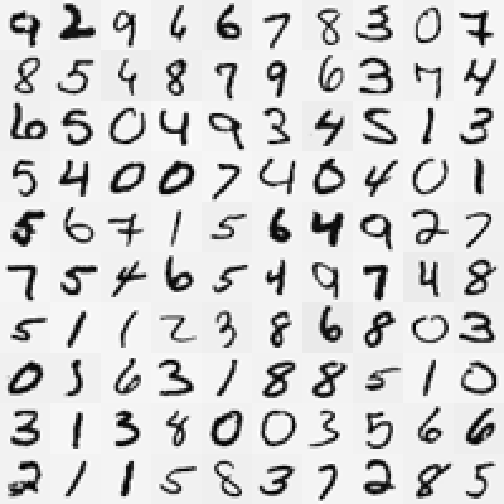
So great, this is what we are trying to classify.
Multiclass classification
In this exercise I’m going to use the code I wrote in the previous post, which should be ready to go out of the box.
For multiclass classification with logistic regression we simply run a mdoel for each possible class, then combine this ensemble of mdoels, and pick the value that has the highest likelihood based on the several models.
Now because the code is well vectorised running ten models together is an absolute breaze. First we define the parameter matrix $\theta$.
Theta <- matrix(
  0,
  ncol = 10,
  nrow = 400
  )
Then use a for loop to generate parameters for each of our ten models
for (i in 1:10) {

  Theta[,i] <- reg_lr(
    X = train,
    y = (train_y == i) * 1,
    theta = Theta[,i],
    lambda = 0
    )

  }
Now we run a logistic regression model using these parameters, which is simply $h_\theta=g(\theta^TX)$ where $g$ is the sigmoid function $g(z)=\frac{1}{1 + e^{-z}}$.
out <- h(Theta,train)

# call the matrixStats package for the rowMaxs function

library(matrixStats)

out_class <- (rowMaxs(out) == out) %>%
  multiply_by(1) %>%
  multiply_by(
    rep(1:10) %>%
      replicate(n = nrow(out)) %>%
      t
    ) %>%
  rowMaxs
The result
That was pretty straightforward. Let’s check the first few predictions against the bitmap plotted earlier:
out_class[1:10]## [1] 9 2 9 6 6 7 8 3 10 7So far so good. Note that zeros are classified as tens to avoid confusion. So how well does the model work on the training data overall?
sum(out_class == train_y)/100## [1] 1So currently the model achieved 100% accuracy with $\lambda = 0$ (the regularisation parameter), i.e. no regularisation at all.
What about a test set?
I’ll wrap this all in a function, then try it on a different subset of the $X$ matrix.
hw_rec <- function(train,test,train_y,test_y,lambda,classes) {

  Theta <- matrix(
    0,
    ncol = classes, # number of classes
    nrow = ncol(train)
    )

  for (i in 1:classes) {

    Theta[,i] <- reg_lr(
      X = train,
      y = (train_y == i) * 1,
      theta = Theta[,i],
      lambda = lambda
      )

    }

  out <- h(Theta,test)

  out_class <- (rowMaxs(out) == out) %>%
    multiply_by(1) %>%
    multiply_by(
      rep(1:10) %>%
        replicate(n = nrow(out)) %>%
        t
      ) %>%
    rowMaxs

  acc <- sum(out_class == test_y)/100

  # Gives output of the predicted classes, the parameters (theta), and the
  # percentage accuracy

  return(
    list(
      class = out_class,
      theta = Theta,
      acc = acc
      )
    )

  }
So repeating the earlier code, I select a different random subset of 100 rows from the $X$ matrix.
y <- "y.csv" %>%
  read.csv(
    header = FALSE
    )

test <- "matrix.csv" %>%
  read.csv(
    header = FALSE
    ) %>%
  cbind(y) %>%
  sample_n(
    100
    ) %>%
  as.matrix

test_y <- test[,401]
test <- test[,-401]
And looping through a range of $\lambda$, how accurately is the model predicting the digits?
lambdas <- c(0.001,0.01,0.1,0.5,1,10)

test_lambda_y <- sapply(
  lambdas,
  function(x) {
      hw_rec(train,test,train_y,test_y,x,10)$acc
    }
  )

test_lambda_y
## [1] 0.76 0.75 0.76 0.77 0.76 0.74So not bad considering the model was trained on a dataset the same size as the test set. With varying levels of regularisation ($\lambda$) the model has between 74% and 77% accuracy.
Next time I’ll define training, test, and cross validation sets with a 60:20:20 split, to improve classification, and better inform my choice of $\lambda$.
sessionInfo()## R version 3.1.2 (2014-10-31)
## Platform: x86_64-unknown-linux-gnu (64-bit)
##
## locale:
## [1] LC_CTYPE=en_GB.UTF-8 LC_NUMERIC=C
## [3] LC_TIME=en_GB.UTF-8 LC_COLLATE=en_GB.UTF-8
## [5] LC_MONETARY=en_GB.UTF-8 LC_MESSAGES=en_GB.UTF-8
## [7] LC_PAPER=en_GB.UTF-8 LC_NAME=C
## [9] LC_ADDRESS=C LC_TELEPHONE=C
## [11] LC_MEASUREMENT=en_GB.UTF-8 LC_IDENTIFICATION=C
##
## attached base packages:
## [1] grid methods stats graphics grDevices utils datasets
## [8] base
##
## other attached packages:
## [1] matrixStats_0.14.0 ucminf_1.1-3 raster_2.3-24
## [4] sp_1.0-15 magrittr_1.5 dplyr_0.2
## [7] testthat_0.9 knitr_1.6
##
## loaded via a namespace (and not attached):
## [1] assertthat_0.1 evaluate_0.5.5 formatR_1.0 lattice_0.20-29
## [5] parallel_3.1.2 Rcpp_0.11.2 stringr_0.6.2 tools_3.1.2