Implementing vectorised logistic regression

I’ve been doing Andrew Ng’s excellent Machine Learning course on coursera. The second exercise is to implement from scratch vectorised logistic regression for classification. Submissions to the exercises have to be made in Octave or Matlab; in this post I give the solution using R.

Andrew Ng uses the algorithm fminunc in Matlab/Octave to optimise the logistic regression solution. In R you can use the optim function, but I have been using the ucminf function provided in the package ucminf. uncminf takes the following arguments:

ucminf(par, fn, gr = NULL, ..., control = list(), hessian=0)

The ones we are interested in are:

Arguments
`par`	Initial estimate of minimum for fn.
`fn`	Objective function to be minimized.
`gr`	Gradient of objective function If `NULL` a finite difference approximation is used.

So I need to define three functions: logistic regression, a cost function, and a function which returns the gradient of that cost. These are defined in the course, helpfully:

Logistic regression is defined as:

$h_{\theta}(x)=g(\theta^{T}x)$

where $g$ is the sigmoid function:

$g(z)=\frac{1}{1+e^{-z}}$

The cost function is given by:

$J(\theta)=\frac{1}{m}\sum^m_{i=1}[-y^{(i)}\log(h_\theta(x^{(i)}))-(1-y^{(i)})\log(1-h_\theta(x^{(i)}))]$

And the gradient of the cost is a vector of the same length as $\theta$ where the $j^{th}$ element (for $j = 0,1,\cdots,n$) is defined as:

$\frac{\delta J(\theta)}{\delta\theta_{j}}=\frac{1}{m}\sum^{m}_{i=1}(h_{\theta}(x^{(i)})-y^{(i)})x^{(i)}_j$

Vectorised logistic regression

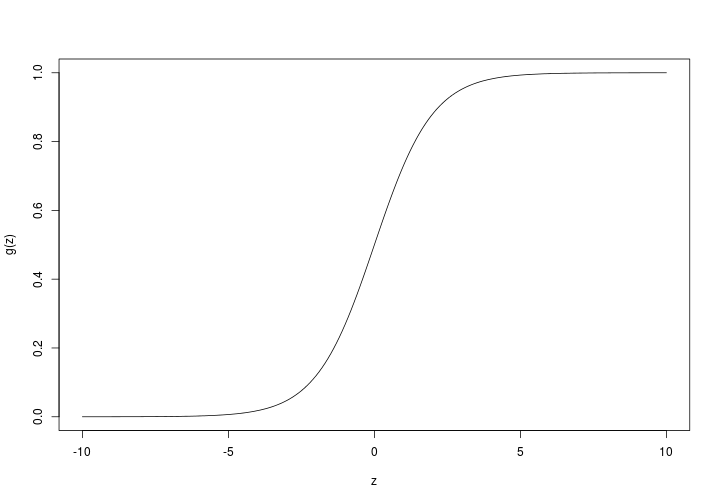
The first step is to implement a sigmoid function:

g <- function(z) {
  
  1 / (1 + exp(-z))
  
  }
 
z <- seq(-10,10,0.1)
 
plot(
  z,
  g(z),
  type = "l"
  )

…and with this function, implementing $h_{\theta}$ is easy:

h <- function(theta,X) {
  
  g(X %*% theta)
  
  }

Cost function and gradient

I’ll start by implementing an only partially vectorised version of the cost function $J(\theta)$:

  J <- function(X, y, theta) {
    (1/length(y)) * sum(-y*log(h(theta,X))-(1-y)*log(1-h(theta,X)))
    }

…and the gradient…

gR <- function(X,y,theta) {
  
  error <- h(theta,X) - y
  delta <- t(X) %*% error / length(y)
  return(delta)
  
  }

Testing it out…

First, I’ll plot the data:

library(dplyr)
library(magrittr)
library(ggplot2)
 
ex2data1 <- "ex2data1.txt" %>%
  read.csv(header=FALSE) %>%
  set_colnames(c("exam_score_1","exam_score_2","admitted"))
 
p <- ex2data1 %>%
  ggplot(
    aes(
      x = exam_score_1,
      y = exam_score_2,
      shape = factor(admitted),
      colour = factor(admitted)
      )
    ) +
  geom_point()+
  xlab("Exam 1 score")+
  ylab("Exam 2 score")
 
p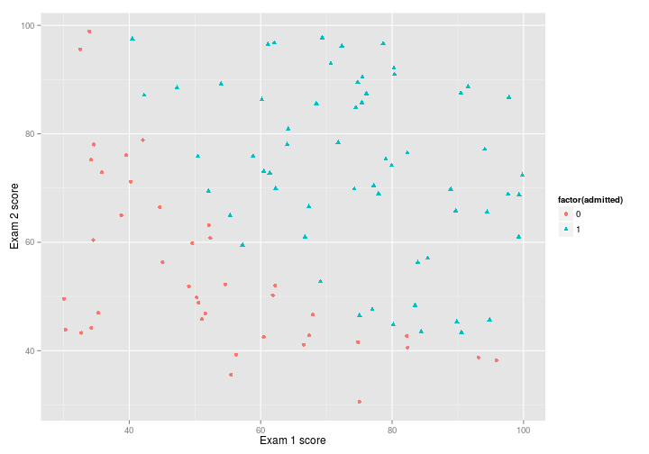

And now try out logistic regression with ucminf:

# arrange the data for the functions
 
theta <- matrix(c(0,0,0), ncol = 1)
X <- ex2data1[,1:2] %>% as.matrix %>% cbind(1,.)
y <- ex2data1[,3] %>% as.matrix
 
library(ucminf)
 
ucminf_out <- ucminf(
  par = theta,
  fn = function(t) J(X, y, t),
  gr = function(t) gR(X, y, t)
  )
 
ucminf_out

## $par
## [1] -25.1613327   0.2062317   0.2014716
## 
## $value
## [1] 0.2034977
## 
## $convergence
## [1] 1
## 
## $message
## [1] "Stopped by small gradient (grtol)."
## 
## $invhessian.lt
## [1] 3314.2043743  -26.3783748  -26.9990573    0.2247604    0.2016443
## [6]    0.2355011
## 
## $info
##  maxgradient     laststep      stepmax        neval 
## 4.236716e-07 2.095353e-05 3.307500e+00 3.200000e+01

So this gives a lot of output. But importantly it gives us three coefficients ($par), the final cost ($value), and that convergence was reached ($convergence).

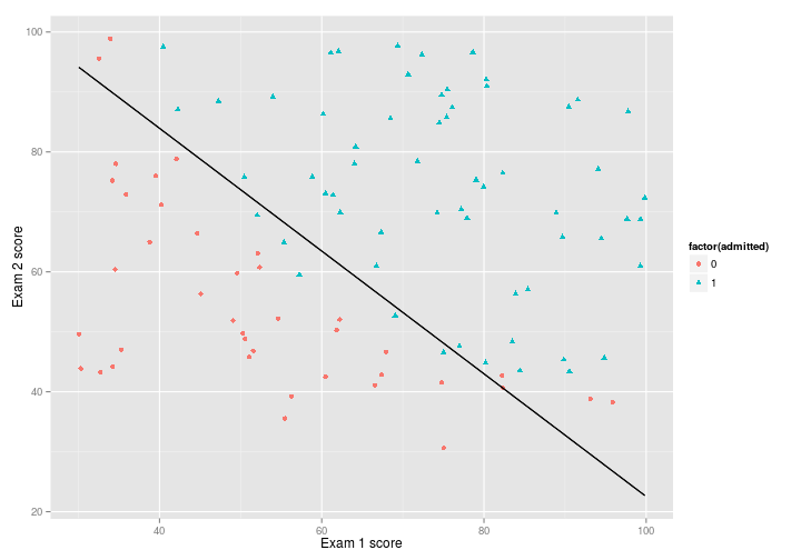
Andrew Ng suggests that the final cost should be 0.203, which is what I get, so it seems to be working, and using $par to plot the decision voundary, we get a pretty good fit:

theta <- ucminf_out$par
 
boundary <- function(x) {
  (-1/theta[3])*(theta[2]*x+theta[1])
  }
 
p + stat_function(
    fun = boundary,
    colour = "black"
    )

Vectorising

There is an excellent post on vectorising these functions on Stack Overflow which gives a better vectorised version of the algorithms above, e.g.:

Jv <- function(X, y, theta) {
  -(1/length(y)) * crossprod(
    c(y, 1 - y), 
    c(log(h(theta,X)), log(1 - h(theta,X)))
    )
  }

It wasn’t immediately clear to me what’s going on here, so I’m going to break this down piece by piece.

First we create two vectors c(y, 1 - y) and c(log(h(theta,X)), log(1 - h(theta,X))) and compute the cross product of them. The first matrix is the concatenation of the $-y$ and $(1-y)$ terms for length $m$ from the equation:

$J(\theta)\frac{1}{m}\sum^m_{i=1}[-y^{(i)}\log(h_\theta(x^{(i)}))-(1-y^{(i)})\log(1-h_\theta(x^{(i)}))]$

The second vector concatenates the remaining terms:

$\text{log}(h_{\theta(x^{(i)})})$

and

$\text{log}(1-h_{\theta(x^{(i)})})$

The crossproduct of these two vectors is essentially the same as $\vec{a}^T\vec{b}$; basically the sum of every value of $\vec{a}$ multiplied by the corresponding value of $\vec{b}$. i.e.: (note that not all of the first vector equal zero: $\vec{a_{(i)}}\neq0$, $\vec{a}\in{0,1}$).

$\begin{bmatrix} 0 & 0 & 0 & \cdots & 0 \end{bmatrix}\begin{bmatrix} -0.6931472 \\ -0.6931472 \\ -0.6931472 \\ \vdots \\ -0.6931472 \end{bmatrix} = -0.6931472$

The $\delta$ function can also be speeded up slightly by employing crossprod instead of t(X) %*% h(theta,X).

gRv <- function(X,y,theta) {
  
  (1 / length(y)) * crossprod(X, h(theta,X) - y)
  
  }

Ok so now that we have some additional vectorisation, let’s look at plugging it into the ucminf function.

ucminf_out_v <- ucminf(
  par = theta,
  fn = function(t) Jv(X, y, t),
  gr = function(t) gRv(X, y, t)
  )
 
ucminf_out_v

## $par
## [1] -25.1613327   0.2062317   0.2014716
## 
## $value
## [1] 0.2034977
## 
## $convergence
## [1] 1
## 
## $message
## [1] "Stopped by small gradient (grtol)."
## 
## $invhessian.lt
## [1] 1 0 0 1 0 1
## 
## $info
##  maxgradient     laststep      stepmax        neval 
## 4.236716e-07 0.000000e+00 3.307500e+00 1.000000e+00

So great, the two are giving the same answer. But it would be interesting to see what the speed increase is like when comparing the non-vectorised, vectorised, and the usual glm method

First let me just check that the glm implementation returns the same parameters:

model <- glm(
  admitted ~ exam_score_1 + exam_score_2,
  family = "binomial",
  data = ex2data1
  )
 
coef(model)

##  (Intercept) exam_score_1 exam_score_2 
##  -25.1613335    0.2062317    0.2014716

Perfect. Now to compare the three I’ll use the excellent rbenchmark package.

library(rbenchmark)
 
benchmark(
  glm = glm(
    admitted ~ exam_score_1 + exam_score_2,
    family = "binomial",
    data = ex2data1
    ),
  ucminf = ucminf(
    par = theta,
    fn = function(t) J(X, y, t),
    gr = function(t) gR(X, y, t)
    ),
  ucminf_vectorised = ucminf(
    par = theta,
    fn = function(t) Jv(X, y, t),
    gr = function(t) gRv(X, y, t)
    ),
  replications = 1000,
  columns = c("test","replications","elapsed")
  )

##                test replications elapsed
## 1               glm         1000   4.022
## 2            ucminf         1000   0.285
## 3 ucminf_vectorised         1000   0.254

So even with a relatively small dataset of just 100 rows, we find that a vectorised linear regression solved using an optimisation algorithm is many times quicker than applying a generalised linear model. Kinda makes it all worthwhile!

Next time I’ll look at implementing regularisation to fit more complicated decision boundaries.

sessionInfo()

## R version 3.1.3 (2015-03-09)
## Platform: x86_64-pc-linux-gnu (64-bit)
## Running under: Ubuntu 14.04.2 LTS
## 
## locale:
##  [1] LC_CTYPE=en_GB.UTF-8       LC_NUMERIC=C              
##  [3] LC_TIME=en_GB.UTF-8        LC_COLLATE=en_GB.UTF-8    
##  [5] LC_MONETARY=en_GB.UTF-8    LC_MESSAGES=en_GB.UTF-8   
##  [7] LC_PAPER=en_GB.UTF-8       LC_NAME=C                 
##  [9] LC_ADDRESS=C               LC_TELEPHONE=C            
## [11] LC_MEASUREMENT=en_GB.UTF-8 LC_IDENTIFICATION=C       
## 
## attached base packages:
## [1] methods   stats     graphics  grDevices utils     datasets  base     
## 
## other attached packages:
## [1] rbenchmark_1.0.0 ucminf_1.1-3     ggplot2_1.0.0    magrittr_1.5    
## [5] dplyr_0.4.1      testthat_0.8.1   knitr_1.9       
## 
## loaded via a namespace (and not attached):
##  [1] assertthat_0.1   colorspace_1.2-5 DBI_0.3.1        digest_0.6.4    
##  [5] evaluate_0.5.5   formatR_1.0      grid_3.1.3       gtable_0.1.2    
##  [9] labeling_0.3     lazyeval_0.1.10  MASS_7.3-39      munsell_0.4.2   
## [13] parallel_3.1.3   plyr_1.8.1       proto_0.3-10     Rcpp_0.11.5     
## [17] reshape2_1.4.1   scales_0.2.4     stringr_0.6.2    tcltk_3.1.3     
## [21] tools_3.1.3

Matt Upson

Recommended reading

Implementing vectorised logistic regression

Vectorised logistic regression

Cost function and gradient

Testing it out…

Vectorising

Matt Upson

Recommended reading

Implementing vectorised logistic regression

Vectorised logistic regression

Cost function and gradient

Testing it out…

Vectorising

You might also enjoy (View all posts)