
K means is one of the simplest algorithms for unsupervised learning. It works iteratively to cluster together similar values in a dataset of one to many dimensions ($X\in\mathbb{R}^{m \times n}$). The algorithmic steps are simple, it relies only on arithmetic means, so it’s pretty simple to understand, but can also be quite powerful. Because it relies on random sampling to initiate the algorithm it can be quite slow however, as there is a need to complete many replications to get a robust result.
K-means features as an exercise in Coursera’s machine learning course, which I am working through. In this post I produce a simple implementation of the K means algorithm in R, and because I’m trying to improve my package writing, I wrap it up into a simple package called knn.
The problem
K-means can be divided into two steps. In a two-dimensional example, given a dataset $X\in\mathbb{R}^{m \times 2}$, the first step is to calculate the closest centroid for each training example $x$. In my implementation, centroids $\{1,…,K\}$ can be assigned manually, or are automatically generated by selecting $K$ random training examples, and setting these as the centroids.
Mathematically, for each training example $x^{i}$ we are minimising
i.e. calculating the Euclidean norm of the vector $x^{(i)}$.
This is very simply achieved through pythagorean trigonometry, and is already implemented in R with norm.
Generate dummy data
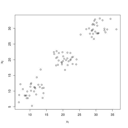
The first step is to generate dummy two dimensional data which will demonstrate the principles well. It’s expedient to functionalise this.
set.seed(1337)
dummy_group <- function(x = 30, mean = 10, sd = 2) {

  cbind(
    rnorm(x, mean, sd),
    rnorm(x, mean, sd)
  )

}

X <- rbind(
  dummy_group(mean = 10),
  dummy_group(mean = 20),
  dummy_group(mean = 30)
)
Which gives us a small dataset with some clear clusters to work with.
plot(
  X,
  xlab = expression(x[1]),
  ylab = expression(x[2])
)
Calculating norms
Calculating norms can be done with base R using norm.
## Note norm only accepts a matrix

norm(as.matrix(c(2,4)),type = "f")
## [1] 4.472136But, the norm function isn’t too useful in the present case, as we really want to vectorise this process, so I use my own function rowNorms:
## Define rowNorms()

rowNorms <- function(x) {

norms <- sqrt(rowSums(x ^ 2))
return(norms)

}
rowNorms works across a matrix, and will return a vector of norms, whilst norm will return the norm of the matrix.
rowNorms(X) %>% str## num [1:90] 16.3 14.1 12.1 21.5 12.1 ...This function is implemented in the knn package.
Calculate distances
So now I can produce a vector of euclidean norms, I can put this into practice for calculating the distance between points $x^i$ and the initial centroids.
In the first instance I will specify some centroids, although as noted, more usual practice is to randomly initiate these from $X$.
So to calculate the distance between some pre-specified centroids and $X$:
## First create a matrix of initial centroids

centroids <- rbind(
c(15, 15),
c(25, 15),
c(25, 35)
)

## Create a matrix with m rows, consisting entirely of the first centroid.

first_centroid <- matrix(
  rep(centroids[1,], nrow(X)),
  ncol = 2,
  byrow = TRUE
  )

diff <- X - first_centroid

distances <- rowNorms(diff)

distances %>% str
## num [1:90] 5.24 8.38 9.19 2.58 9.06 ...Rather than repeating this for all three initial centroids, I’ve wrapped this up into a function.
Here knn::find_group() calculates the closest centroid and returns this as a vector of values ${1,..,K}$, where $K$ is the number of centroids.
groups <- find_group(X, centroids = centroids)

## Returns a vector of groups based on proximity to the initial centroids

groups %>% str
## int [1:90] 1 1 1 1 1 1 1 1 1 1 ...Calculate centroids
The next step of the process is to now calculate the new centroid from the groups that were established in the previous step.
Again, this is qute a simple thing to code.
I achieved it by sequentially subsetting $X$ by $k$, and outputting the new centroids in a matrix $Y\in\mathbb{R}^{K \times n}$.
I’ve wrapped this step into a function called centroid_mean().
Y <- centroid_mean(X, groups)With the centroids calculated, now is a good chance to plot again, and check the sanity of the new centroids.
I’ve written a function plot_knn() to do this (it would make sense to roll this up into a plot method one day…).
Start with the original centroids…
plot_knn(X, centroids)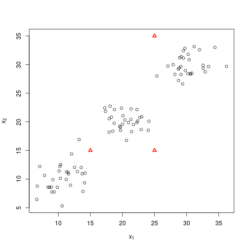
And now with the new centroids…
plot_knn(X, Y)
Not bad, so it looks things are moving in the right direction, and with one further iteration, it looks like we are pretty close to the original centroids.
groups1 <- find_group(X, centroids = Y)
Y1 <- centroid_mean(X, groups1)
plot_knn(X, Y1)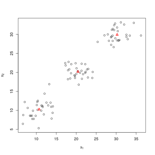
I could keep on going manually, but I have already implemented the whole process in the function knn(). So I’ll try that instead, this time randomly initiating the centroids.
# Set seed to make results reproducible
set.seed(1)
foo <- knn(X, k = 3)
plot_knn(X, foo$centroids, foo$groups)
Great, so what are the final centroids?
foo$centroids %>% round## [,1] [,2]
## [1,] 11 10
## [2,] 30 30
## [3,] 20 20…which as you’ll remember were the starting values about which I generated the normal distributions. Of course, it wouldn’t normally be possible to assess the success of the algorithm so easily, and note that the order of the centroids has changed, although this doesn’t matter.
A harder test
I’ll try again with a more difficult example. Here I am still relying on three normally distributed clusters about the same centroids, but I specify a much greater standard deviation, so it is much more difficult with the human eye alone to separate the clusters. I’ll specify $x = 100$ so that the algorithm has more data to work with.
X <- rbind(
  dummy_group(x = 100, mean = 10, sd = 8),
  dummy_group(x = 100, mean = 20, sd = 8),
  dummy_group(x = 100, mean = 30, sd = 8)
)

plot(
  X,
  xlab = expression(x[1]),
  ylab = expression(x[2])
    )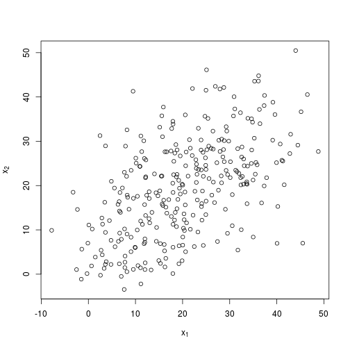
Hard to see three distinct clusters…now what the algorithm makes of it.
Again, I use the knn() function which takes the leg work out of the programming.
In the example below I also set a seed which will make the results reproducible. As I noted in the pre-amble, the solutions from K-means are dependent on the initial centroids, so it is usual practice to repeat the process many times, and then choose the group that has the highest probability.
I’ve not yet implemented this repetition in knn yet (and probably won’t go that far), so for now I will use set.seed() to demonstrate the ideal and not-so-ideal outcomes.
## set.seed(2) for a good outcome

set.seed(2)
foo <- knn(X)

plot_knn(X, foo$centroids, foo$groups)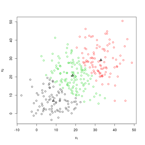
foo$centroids %>% round## [,1] [,2]
## [1,] 9 7
## [2,] 33 29
## [3,] 18 21So we’re a little bit out this time after 3 steps, but not too far. This could probably be improved by setting a more precise endpoint, which at present has a very simplistic implementation.
So what happens if I change the seed?
set.seed(100)
bar <- knn(X)
plot_knn(X, bar$centroids, bar$groups)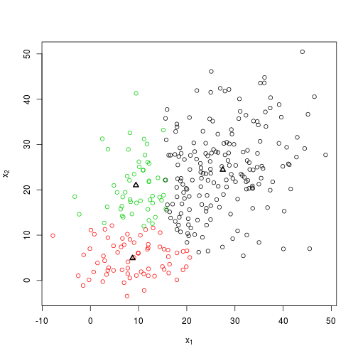
bar$centroids %>% round## [,1] [,2]
## [1,] 27 24
## [2,] 9 5
## [3,] 9 21So the solution given by the algorithm has changed, and this highlights one of the issues with K-means: it can be very dependent on the initial location of centroids.
This is why it is usual to repeat the process many times, then essentially average the results.
I haven’t gone that far with my simple implementation, but the in-built implementation in base R (kmeans) does include an argument nstarts which will give you $n$ possible scenarios.
So how well does kmeans() perform in the current scenario? Well not vastly different it turns out.
foobar <- kmeans(X, centers = 3, nstart = 1)
plot_knn(X, foobar$centers, foobar$cluster)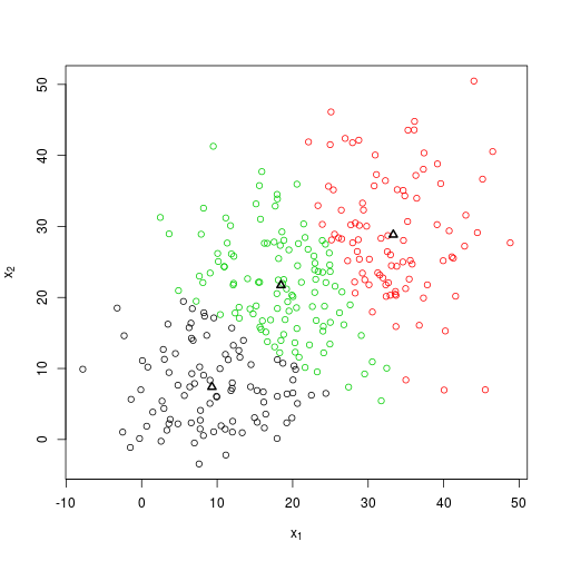
foobar$centers %>% round## [,1] [,2]
## 1 9 7
## 2 33 29
## 3 18 22What about the improvement with additional replications?
foobar <- kmeans(X, centers = 3, nstart = 1000)
plot_knn(X, foobar$centers, foobar$cluster)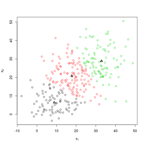
foobar$centers %>% round## [,1] [,2]
## 1 9 6
## 2 18 21
## 3 33 29At two decimal places, there is only a small difference between the final centroids, and those produced by only a single repetition using kmeans().
Of course I should note that kmeans() uses a more complicated (and more accurate) algorithm than the simplified implementation I have used in knn.
A more interesting application
One of the ways that K-means can be used is for image compression. Images are just arrays of values, which code for intensity. A grayscale image requires just a single matrix, while a colour image typically requires three matrices. By clustering similar colour values in an image, we can compress an image by reducing the number of colours required to render it. Note that png images may also have a fourth channel which codes for alpha, or transparency.
I use the jpeg package to load and image, in an example inspired by both Markus Gesmann and the Coursera machine learning course, but using my own implementation of K-means.
First I load in a holiday snap in glorious full colour…
library(jpeg)

img <- readJPEG(source = "figures/2015-11-11-knn.jpeg")

## Get dimensions of image

dm <- dim(img)

## Create a matrix of x and y pixel positions and intensity values, and convert
## into rgb

img_df <- data_frame(
  x = rep(1:dm[2], each = dm[1]),
  y = rep(dm[1]:1, dm[2]),
  red = as.vector(img[,,1]),
  green = as.vector(img[,,2]),
  blue = as.vector(img[,,3]),
  cols = rgb(red, green, blue)
)

## Plot the original image

plot(
  y ~ x,
  data = img_df,
  main = "Venice canal (original)",
  col = cols,
  pch = ".",
  axes = FALSE,
  xlab = "",
  ylab = ""
)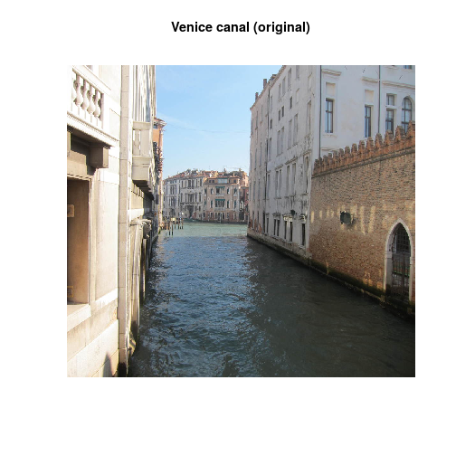
Now the same image again after clustering the colours into sixteen clusters.
## Get clusters from the three intensity values.

kmeans16 <- img_df %>%
  select(red:blue) %>%
  knn(k = 16)

## Convert clusters into rgb values, and append as column to img_df

img_df$cols16 <- rgb(kmeans16$centroids[kmeans16$groups,])

## Plot the image again, this time using the new clustered colours.

plot(
  y ~ x,
  data = img_df,
  main = "Venice canal (16 colours)",
  col = cols16,
  pch = ".",
  axes = FALSE,
  xlab = "",
  ylab = ""
)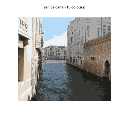
So it works! And whilst I have not attempted to calculate the resulting image compression, the reduction in possible colour values should lead to a pretty considerable reduction in the file size.
I’m not going to develop this package any further, because far better implementations are already out there, but it was a good exercise to learn more about K-means, and package writing in R.
sessionInfo()## R version 3.2.3 (2015-12-10)
## Platform: x86_64-pc-linux-gnu (64-bit)
## Running under: Ubuntu 14.04.3 LTS
##
## locale:
## [1] LC_CTYPE=en_GB.UTF-8 LC_NUMERIC=C
## [3] LC_TIME=en_GB.UTF-8 LC_COLLATE=en_GB.UTF-8
## [5] LC_MONETARY=en_GB.UTF-8 LC_MESSAGES=en_GB.UTF-8
## [7] LC_PAPER=en_GB.UTF-8 LC_NAME=C
## [9] LC_ADDRESS=C LC_TELEPHONE=C
## [11] LC_MEASUREMENT=en_GB.UTF-8 LC_IDENTIFICATION=C
##
## attached base packages:
## [1] methods stats graphics grDevices utils datasets base
##
## other attached packages:
## [1] knn_0.1.3 jpeg_0.1-8 dplyr_0.4.3 testthat_0.11.0
## [5] knitr_1.11
##
## loaded via a namespace (and not attached):
## [1] Rcpp_0.12.2 digest_0.6.8 crayon_1.3.1 assertthat_0.1
## [5] R6_2.1.1 DBI_0.3.1 formatR_1.2.1 magrittr_1.5
## [9] evaluate_0.8 stringi_1.0-1 lazyeval_0.1.10 tools_3.2.3
## [13] stringr_1.0.0 parallel_3.2.3 memoise_0.2.1