About a year into the PhD thesis writing process, I decided to make a switch from a widely known WhatYouSeeisWhatYouGet word processor, into $\LaTeX$. It all started with a black line at the bottom of the page. It appeared one day while I was writing a riveting chapter on soil carbon, and looked like a border on top of the footer. I don’t know where it came from, and no matter what I tried, I couldn’t get rid of it. No amount of fiddling, copying and pasting into new documents, or inappropriate language worked- I was stuck with this line on every single page of my Thesis.
So, having written a couple of project reports in $\LaTeX$, I decided to take the plunge, and began to write using the package knitr by Yihui Xie to blend my R code with $\LaTeX$ in one document.
Some lessons learnt
So several months down the line, thesis submitted, corrected, PhD awarded, I feel that I’m in a good position to give some advice to those considering setting out on a similar $\LaTeX$ journey. I made a lot of early mistakes, which I was subsequently stuck with; writing them here is a kind of catharsis, that perhaps someone will be able to learn from.
Lesson 1: Don’t use someone else’s template
(or at least, use the simplest template you can find)
I’m aware that this is perhaps counter-intuitive advice, so I’ll explain my reasons. I started out early on using the classicthesis template by Andre Miede (Andre, I owe you a postcard). It looks great, and it’s designed to follow all sort of typographical rules that we, as scientists, are likely to be oblivious to.
The problem is, that it is quite complicated. There is a lot of code, and there are a lot of package dependencies that are called, and even having written a thesis with this template I have to confess, I don’t know what they all do. That’s fine if it all works (although I don’t like the blackbox idea - this after all is why I want to use $\LaTeX$), but occasionally you will run into errors.
This isn’t the fault of the author, but may be due to updates in package dependencies and resulting conflicts - frankly in many cases I still don’t know what the causes were because in those last frantic weeks of getting things together I had time only to hack through and get things working, not to diagnose and fix the problems properly.
If I was doing it again, I would have written my own template from scratch, or started with the simplest template I could find written by someone else, and adapted it to my own means, rather than jumping into a more complicated (if lovely) template like classicthesis. Bear in mind - this was my first significant $\LaTeX$ document; and it is to people in a similar situation that I offer this advice.
Lesson 2: Use knitr
If you are going down the reproducible route like I was, and blending your R code with your $\LaTeX$, use knitr, not sweave.
Knitr is awesome. Spend the time learning the features like hooks. These allow you to write commands that will can automatically be executed whenever you create a code chunk, which can be great for things you do repetitively, like plotting:
library(knitr)

# Set up two plots in one pane

knit_hooks$set(
  plot.mar = function(before, options, envir) {
    if (before) par(
      mfrow = c( 1, 2)
      )
    }
  )
Calling this command in the header of the code chunk with plot.mar = TRUE will apply the function to the chunk:
foo <- rnorm(1:1000)
hist(foo)
plot(density(foo))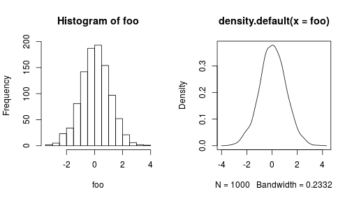
Learning to use the opts_chunk$set() and opts_knit$set() can also save a lot of repetition.
The cache=TRUE option is also very useful when running the analysis becomes a bottleneck in the compilation process. Using cache will save out the results of the analysis, and just recall the cached object each time you run the chunk.
Be aware that this can lead to problems if, for instance, the data being passed to a chunk has changed, but the code in the chunk itself has not. Without a change in the chunk itself, knitr will not re-evaluate the chunk, and it can lead to a lot of confusion.
Automatically creating tables can be made relatively painless with the xtable package, which has a load of options to allow you to customize your tables.
Combined with dplyr, the two are very flexible. You’ll need to specify results="asis" to get this to display properly in a .Rnw document.
library(dplyr)
library(xtable)

# Note that \pm is escaped for R with an additional slash \

errors <- function(x,y) {
  paste("$", sprintf("%.2f", x), "\\pm", sprintf("%.2f", y), "$", sep = "")
  }

iris_data <- iris %>%
  dplyr::group_by(
    Species
    ) %>%
  dplyr::summarise_each(
    funs(mean, sd)
    ) %>%
  dplyr::transmute(
    species = Species,
    Sepal.Length = errors(Sepal.Length_mean,Sepal.Length_sd),
    Sepal.Width = errors(Sepal.Width_mean,Sepal.Width_sd),
    Petal.Width = errors(Petal.Width_mean,Petal.Width_sd)
    )


iris_table <- iris_data %>%
  xtable(
    caption = "Summary of the Iris data showing mean $\\pm$ SD",
    align = c("r","r","l","l","l"),
    label = "tab:iris_table"
    )
Now this must be wrapped up in a call to print.xtable which allows additional options to be specified. add.to.row is particularly useful, as it allows you to customise table headers. You need to supply it with a list containing a list called pos containing a list of row numbers, and command which includes a character vector of the $\LaTeX$ commands which will be inserted in each equivalent row.
print.xtable(
  iris_table,
  include.rownames = FALSE,
  include.colnames = FALSE,
  caption.placement = "top",
  table.placement = "bth",
  booktabs = TRUE,
  sanitize.text.function = function(x) print(x), # must hack this to allow the printing of \pm
  add.to.row =
    list(
      pos = list(0,0),
      command = c(
        "& \\multicolumn{2}{c}{Sepal} & \\multicolumn{1}{c}{Petal} \\\\ \\cline{2-4}",
        "Species & Length & Width & Width \\\\"
        )
      )
  )
## [1] "setosa" "versicolor" "virginica"
## [1] "$5.01\\pm0.35$" "$5.94\\pm0.52$" "$6.59\\pm0.64$"
## [1] "$3.43\\pm0.38$" "$2.77\\pm0.31$" "$2.97\\pm0.32$"
## [1] "$0.25\\pm0.11$" "$1.33\\pm0.20$" "$2.03\\pm0.27$"
## % latex table generated in R 3.2.0 by xtable 1.7-4 package
## % Mon May 25 12:00:55 2015
## \begin{table}[bth]
## \centering
## \caption{Summary of the Iris data showing mean $\pm$ SD}
## \label{tab:iris_table}
## \begin{tabular}{rlll}
## \toprule
## & \multicolumn{2}{c}{Sepal} & \multicolumn{1}{c}{Petal} \\ \cline{2-4} Species & Length & Width & Width \\ \midrule
## setosa & $5.01\pm0.35$ & $3.43\pm0.38$ & $0.25\pm0.11$ \\
## versicolor & $5.94\pm0.52$ & $2.77\pm0.31$ & $1.33\pm0.20$ \\
## virginica & $6.59\pm0.64$ & $2.97\pm0.32$ & $2.03\pm0.27$ \\
## \bottomrule
## \end{tabular}
## \end{table}Lesson 3: But…maybe don’t use knitr
So if you are dead set on going to fully reproducible route, definitely definitely use knitr. If you are still exploring options, then I would think carefully about whether to make your document completely reproducible in this way.
Don’t get me wrong - I went for the completely reproducible route, and if I was doing it again now I would do the same. If I was advising my earlier self without the experience I have 3 years down the line, I might have said not to bother going fully reproducible, and produced my R code apart from the $\LaTeX$.
There are a couple of reasons for this. Firstly, when you are in the final panic stages of PhD production, you may want to avoid the complexity of having to debug two languages at the same time, especially if both are relatively new to you. And for sure, debugging R code in a reproducible document is much more challenging.
Part of the problem is that the flow of your code may no longer be linear. It might be the case that I want to quote the output of a bit of analysis before I would logically site the analysis chunk (probably in the results section), but you also have a chunk printing that analysis in the results section too. It’s not a major issue, but it does require some thought early on. So if you are going to do it - get your workflow right. Get in the habit of loading data from files as normal, then saving out intermediate analysis steps to .Rdata or .Rds files, so that these can quickly be recalled to other chunks if required.
Update 2015-05-10: Yihui gives some solutions to this problem by allowing you specify dependencies between chunks in the chunk options. This page is very worth a read.
Lesson 4: Manage your dependencies
Despite having produced my thesis in a ‘fully reproducible’ format, less than a year later, I am now unable to reproduce it. Oooops.
Why? Because packages (and I’m predominantly talking R packages) have been updated, and have my old code is not compatible with the new versions.
How did this happen?
I simply didn’t manage my dependencies well.
At the very least I should have recorded which versions of R packages I had used at the time when I was developing the code.
This can be as easy as a call to sessionInfo() at the time of compiling - or better still, include this in an appendix so you know for sure which versions of the R packages you were using when you compiled.
sessionInfo()## R version 3.2.0 (2015-04-16)
## Platform: x86_64-unknown-linux-gnu (64-bit)
## Running under: Ubuntu 14.04.2 LTS
##
## locale:
## [1] LC_CTYPE=en_GB.UTF-8 LC_NUMERIC=C
## [3] LC_TIME=en_GB.UTF-8 LC_COLLATE=en_GB.UTF-8
## [5] LC_MONETARY=en_GB.UTF-8 LC_MESSAGES=en_GB.UTF-8
## [7] LC_PAPER=en_GB.UTF-8 LC_NAME=C
## [9] LC_ADDRESS=C LC_TELEPHONE=C
## [11] LC_MEASUREMENT=en_GB.UTF-8 LC_IDENTIFICATION=C
##
## attached base packages:
## [1] methods stats graphics grDevices utils datasets base
##
## other attached packages:
## [1] xtable_1.7-4 dplyr_0.4.1 checkpoint_0.3.10 testthat_0.9.1
## [5] knitr_1.10
##
## loaded via a namespace (and not attached):
## [1] lazyeval_0.1.10 assertthat_0.1 magrittr_1.5 formatR_1.2
## [5] parallel_3.2.0 DBI_0.3.1 tools_3.2.0 Rcpp_0.11.6
## [9] stringi_0.4-1 stringr_1.0.0 evaluate_0.7I didn’t do this, and although some packages were completely up-to-date, so I can work out which packages were the latest at that time, some packages were not. My bad, I learnt the lesson.
There are in fact two (well three) very nice solutions to this problem:
- packrat
- checkpoint
- docker
Packrat solves this problem by packaging up your library with your RStudio project, so that you can save it and take it with you wherever you go. Simple, and great if you are going to be working offline. The downside is, if you are working with many packages, and you want to send it to a friend, this might add many megabytes to the size of what you are sending.
Checkpoint takes a cloud based approach to the same problem.
By calling checkpoint("2015-04-20") checkpoint will download the most up-to-date versions of the packages I am using available on 2015-04-20, and create a separate library.
This is a nice solution because it only requires one call to a package, and one line of code to fix the issue for anyone.
I now use checkpoint with every project I do, and particularly when writing papers.
Docker is something altogether different, and probably represents the future. Docker allows you to run code in a container (think docking container) which can be run cross-platform. These containers can be set up in advance, pushed to a repository and shared, and can have all the dependencies you need (in R and everything else) all ready to go. There are containers for R already (the Docker R project is called ‘Rocker’) and there are a number of containers available, including the aptly named ‘hadleyverse’.
Lesson 5: Use version control
Now this is something we should all be doing if we are working with R, but is especially pertinent when writing a large document in $\LaTeX$. Install git, brave the learning curve, and you will not regret it. Version control with git allows you to save snapshots of your work when you make important edits, and importantly, lets you roll back to previous edits if you break it.
It is also great for sharing code and collaborating with github or bitbucket, and others. I’m not going to say any more about git and version control, because there is so much information out there about it already.
My advice is use it, sooner rather than later…and consider using a new line for every sentence, otherwise git will report changes at the paragraph level, not the individual sentence.
Concluding remarks
Of course, perhaps the greatest challenge you may face when switching to $\LaTeX$ is convincing your supervisor to accept a pdf copy. I was quite lucky in that my supervisor was happy to make edits either on paper, or onto a pdf. For others I have had to resort to running the pdf through an online converter to allow them to make edits; I would then incorporate the edits from this version into $\LaTeX$ manually.
It is not inconceivable that supervisors might be convinced to learn $\LaTeX$, and if you can do this there are online tools which aid collaboration like ShareLaTeX and Overleaf, which allow real-time compilation. But of course by this point I hope you will be working with git which also makes collaboration very simple.
So I hope some of the above will be useful to someone. These are some of the words of advice I would have given to my younger self and to anyone starting out on a PhD, along with a heartfelt ‘good luck’.