Linear regression with gradient descent

For the implementation of gradient descent for linear regression I draw from Digithead’s blog post.

Andrew Ng defines gradient descent for linear regression as:

$\begin{multline} \text{repeat until convergence} \{\\ \theta_0:=\theta_0 - \alpha\frac{1}{m}\sum_{i=1}^{m}(h_{\theta}(x^{(i)})-y^{(i)})\\ \theta_1:=\theta_1 - \alpha\frac{1}{m}\sum_{i=1}^{m}(h_{\theta}(x^{(i)})-y^{(i)})\cdot x^{i}\\ \} \end{multline}$

Where $\alpha$ is the training rate, $m$ is the number of training examples, and the term on the right is the familiar squared error term after multiplication with the partial derivative $\frac{\delta}{\delta\theta_0}$ or $\frac{\delta}{\delta\theta_1}$ as appropriate.

Digithead’s implementation of this is quite slick, and it took me a while to get my head around the vectorised implementation, so I will break it down here, for my own memory if nothing else:

# Start by loading the data and splitting into vectors
 
"ex1data1.txt" %>% 
  read.csv(header =  FALSE) %>%
  set_colnames(c("x","y")) -> ex1data1
 
X <- cbind(1,matrix(ex1data1$x))
 
y <- ex1data1$y

To run linear regression as a matrix multiplication it is necessary to add a column of ones, so that $x_0 = 1$. This means that when matrix $X$ is multiplied by the parameter matrix $\theta$, the intercept $\theta_0=\theta_0\times1$. i.e.:

$\begin{bmatrix} x^0_0 & x^1_0 \\ x^0_1 & x^1_1 \\ x^0_2 & x^1_2 \\ \vdots & \vdots \\ x^0_3 & x_m \end{bmatrix}\times\begin{bmatrix} \theta_0 \\ \theta_1 \end{bmatrix}=\begin{bmatrix} \theta_0 + (x^1_0\times\theta_1) \\ \theta_0 + (x^1_1\times\theta_1) \\ \theta_0+ (x^1_2\times\theta_1) \\ \vdots \\ \theta_0 + (x^1_m\times\theta_1) \end{bmatrix}\approx a+bx$

We define the usual squared error cost function:

$J(\theta_0,\theta_1)=\frac{1}{2m}\sum_{i=1}^{m}(h_\theta(x)-y)^2$

Except that in Digithead’s implementation below $h_\theta$ is defined by the matrix multiplication of $X$ and $\theta$ as described above, and rather than multiplying by $\frac{1}{2m}$, he divides by $2m$.

cost <- function(X, y, theta) {
  sum( (X %*% theta - y)^2 ) / (2*length(y))
}

Alpha is set at a low number initially, and the number of iterations set to 1000.

alpha <- 0.01
num_iters <- 1000

A vector and a list are initialised to handle the history of the cost function $J(\theta_0,\theta_1)$ and the parameters $\theta$ at each iteration.

cost_history <- double(num_iters)
theta_history <- list(num_iters)

The coefficients for regression are initialised to zero

theta <- matrix(c(0,0), nrow = 2)

Finally, the gradient descent is implemented as a for loop:

for (i in 1:num_iters) {  
  error <- (X %*% theta - y)
  delta <- t(X) %*% error / length(y)
  theta <- theta - alpha * delta
  cost_history[i] <- cost(X, y, theta)
  theta_history[[i]] <- theta
}

This makes a reasonably large jump, so I’ll break down each line of this loop, for my own understanding.

Recall that Andrew Ng defines the final algorithm for gradient descent for linear regression to be:

The first and second lines of the loop handle the term $(h_{\theta}(x^{(i)})-y^{(i)})\cdot x^{(i)}$. The first line:

error <- (X %*% theta - y)

does our linear regression by matrix multiplication, as mentioned above. The second line:

delta <- t(X) %*% error / length(y)

does both the sum ($\sum_{i=1}^{m}$) and the element-wise multiplication denoted by the $\cdot x^{(i)}$. In the latter case this takes every single error (predicted - observed) score from the error function and multiplies it by the transpose $X$ (t(X)), which includes $x_0=1$.

To give a snippet of this calculation from the first iteration:

$\begin{bmatrix} 1.00 & 1.00 & \cdots & 1.00 \\ 6.11 & 5.53 & \cdots & 5.44 \end{bmatrix}\begin{bmatrix} -17.59 \\ -9.13\\ \vdots \\ -0.617 \end{bmatrix}=\begin{bmatrix} (1.00\times-17.59)+(1.00\times-9.13)+\cdots+(1.00\times-0.617) \\ (6.11\times-17.59)+(5.53\times-9.13)+\cdots+(5.44\times-0.617) \end{bmatrix}$

So this will end with a two dimensional vector (or a $2\times1$ dimensional matrix) delta$\in\mathbb{R}^{2}$. The end of this line divides by the length of the vector y, or in the notation that I have been using so far: $m$, and this is in place of multiplying by $\frac{1}{m}$.

The third line of the loop:

theta <- theta - alpha * delta

updates $\theta$ using the learning rate $\alpha$ multiplied by delta, whilst the next line:

cost_history[i] <- cost(X, y, theta)

applies the sum of squares cost function to the parameters $\theta$ following the update, and saves this out to the double-precision vector cost_history initialised earlier.

Finally, the last line of the code saves out the parameter vector $\theta$ to the list theta_history. The loop then repeats.

So let’s run it and see what happens…and just out of interest, I have included a call to system.time so we can measure how long it takes.

system.time(
for (i in 1:num_iters) {  
  error <- (X %*% theta - y)
  delta <- t(X) %*% error / length(y)
  theta <- theta - alpha * delta
  cost_history[i] <- cost(X, y, theta)
  theta_history[[i]] <- theta
}
)

##    user  system elapsed 
##   0.046   0.000   0.046

print(theta)

##           [,1]
## [1,] -3.241402
## [2,]  1.127294

We can check these values using the built in regression function in R which uses the normal equation, also with a call to system.time.

system.time(
model <- lm(ex1data1$y~ex1data1$x)
)

##    user  system elapsed 
##   0.002   0.000   0.003

print(model)

## 
## Call:
## lm(formula = ex1data1$y ~ ex1data1$x)
## 
## Coefficients:
## (Intercept)   ex1data1$x  
##      -3.896        1.193

So interestingly this shows us that the gradient decsent run for 1000 iterations has stopped short of finding the correct answer, and also took much longer. This may mean that $\alpha$ is too small, or that there were not enough iterations. The answer is close, but still not quite the same as the answer derived from the noraml equation:

plot(ex1data1)
abline(a=theta[1],b=theta[2])
abline(model,col="red",lty=2)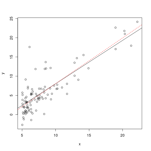

Plotting $J(\theta_0,\theta_1)$ for each iteration would indicate that we had not yet minimised $J(\theta_0,\theta_1)$, and that it is continuing to fall with each further iteration:

par(mfrow = c(1,2))
 
plot(
  cost_history, 
  type = "l", 
  ylab = expression(J(theta[0],theta[1])),
  xlab = "Iteration"
  )
 
plot(
  cost_history, 
  type = "l", 
  ylab = expression(J(theta[0],theta[1])),
  xlab = "Iteration",
  xlim = c(900,1000),
  ylim = c(4.515,4.535)
  )

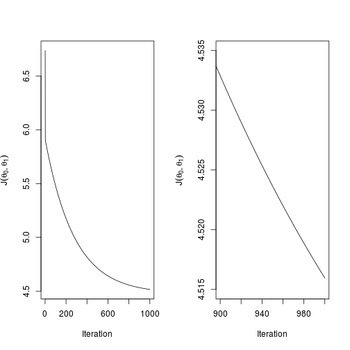
The right hand plot just zooms in on the left hand plot, at the very end of the curve, so we can see that it is still dropping at quite a pace.

This time I try gradient descent again with having rolled the code into a self-contained function to take arguments and follow the notation that Andrew Ng has stuck to in the machine learning course. In addition, the cost function has been changed to the vectorised form:

$J(\theta)=\frac{1}{2m}(X\theta-\vec{y})^T(X\theta-\vec{y})$

grad <- function(alpha, j, X, y, theta) {
  
#   J <- function(X, y, theta) {
#     sum( (X %*% theta - y)^2 ) / (2*length(y))
#     }
  
  # The cost function vectorises to:
  
  J <- function(X, y, theta) {
    (1/2*length(y)) * t((X %*% theta - y)) %*% (X %*% theta - y)
    }
  
  theta_history <<- matrix(nrow = j, ncol = ncol(X) + 1)
  
  for (i in 1:j) {  
    error <- (X %*% theta - y)
    delta <- t(X) %*% error / length(y)
    theta <- theta - alpha * delta
    theta_history[i,] <<- c(theta,J(X, y, theta))
    
    if (i > 1) {
      
      # Here I define a function to calculate when we have roughly reached
      # convergence.
      
      if (
        isTRUE(
          all.equal(
            theta_history[i,3],
            theta_history[i-1,3]
            #tolerance = # can set a tolerance here if required.
              )
          )
        ) {
        
        theta_history <<- theta_history[1:i,]
        break
        
        }
      }
    
    }
  
  list(
    theta = theta,
    cost = theta_history[i,3],
    iterations = i
    )
  
  }

So we define $\theta$ and then save it out to the object out, this time specifying many more iterations.

theta <- matrix(c(0,0), nrow = 2)
out <- grad(0.02, 3000, X, y, theta) %>% print

## $theta
##           [,1]
## [1,] -3.885737
## [2,]  1.192025
## 
## $cost
## [1] 42123.91
## 
## $iterations
## [1] 1656

Now let’s plot it, along with $J(\theta_0,\theta_1)$.

par(mfrow=c(1,2))
 
plot(ex1data1)
abline(a=out[[1]][1],b=out[[1]][2])
abline(model,col="red",lty=2)
 
plot(
  cost_history,
  xlab="Iteration",
  ylab=expression(J(theta[0],theta[1])),
  type="l"
  )

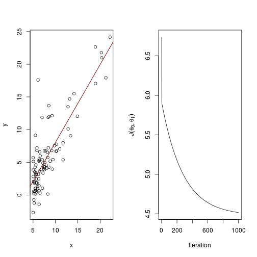
So this time it appears to converge, although it took many iterations to get here. Some adjustment of the learning rate would probably bring this down.

Matt Upson

Recommended reading

Linear regression with gradient descent

Matt Upson

Recommended reading

Linear regression with gradient descent

You might also enjoy (View all posts)