Multivariate linear regression

So this time I’m going to implement gradient descent for multivariate linear regression, but also using feature scaling. I’m using teh dataset provided in the machine learning course, which describes the cost of houses based on two parameters: the size in square feet, and the number of rooms, and giving prices in dollars.

First I’ll load the data and take a look at it.

library(dplyr)
library(magrittr)
library(ggplot2)
 
"ex1data2.txt" %>% 
  read.csv(
    header = FALSE, 
    col.names = c("size","n_rooms","price")
    ) %>%
  dplyr::mutate(
    n_rooms = factor(n_rooms)
    ) -> house_prices
 
 
house_prices %>% head

##   size n_rooms  price
## 1 2104       3 399900
## 2 1600       3 329900
## 3 2400       3 369000
## 4 1416       2 232000
## 5 3000       4 539900
## 6 1985       4 299900

So we have two $x$’s: size and n_rooms

Let’s also plot it out of interest:

p <- house_prices %>%
  ggplot(
    aes(
      x = size,
      y = price,
      colour = n_rooms
      )
    ) +
  geom_point()+
  scale_x_continuous(expression(Size~(ft^2)))+
  scale_y_continuous(
    "Price (1000 $)", 
    breaks = seq(2e+05,7e+05,1e+05), 
    labels = seq(20,70,10)
    )
 
p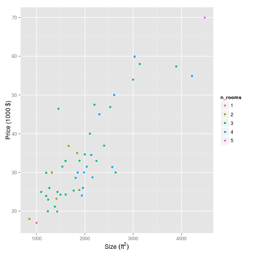

Feature normalisation/scaling

To copy the exercise document:

Your task here is to complete the code in featureNormalize.m to

Subtract the mean value of each feature from the dataset.

After subtracting the mean, additionally scale (divide) the feature values by their respective “standard deviations.”

and in the file featureNormalize.m provided with the course material, we get:

First, for each feature dimension, compute the mean of the feature and subtract it from the dataset, storing the mean value in mu. Next, compute the standard deviation of each feature and divide each feature by it’s standard deviation, storing the standard deviation in sigma.

Note that X is a matrix where each column is a feature and each row is an example. You need to perform the normalization separately for each feature.

I’ll have a go at implementing that in R.

feature_scale <- function(x) {
  
  # Convert all factors to numeric
  # Note that this will also allow the conversion of string features
  
  for (i in 1:ncol(x)) {
    x[,i] %>% as.numeric -> x[,i]
    }
  
  # Set up matrices to take outputs
  
  mu <- matrix(nrow = 1, ncol = ncol(x))
  sigma <- matrix(nrow = 1, ncol = ncol(x))
  scaled <- matrix(nrow = nrow(x), ncol = ncol(x))
  
  # Define feature scaling function
  
  scale <- function(feature) {
    (feature - mean(feature)) / sd(feature)
    }
  
  # Run this for each of the features
  
  for (i in 1:ncol(x)) {
    
    mu[,i] <- mean(x[,i])    
    sigma[,i] <- sd(x[,i])
    scaled[,i] <- scale(x[,i])
    
    }
  
  # And output them together as a list
  
  list(
    mu = mu,
    sigma = sigma,
    scaled = scaled
    )  
  }

Ok so let’s try this on our features in the housing dataset.

scaled_features <- feature_scale(house_prices[,-3])

We can have a look to see what this has done to our values. Originally the ranges for the features were:

house_prices %$% size %>% range

## [1]  852 4478

and

house_prices %$% n_rooms %>% as.character %>% as.numeric %>% range

## [1] 1 5

…so quite a difference.

After feature scaling these ranges are:

scaled_features %$% scaled %>% extract(,1) %>% range

## [1] -1.445423  3.117292

and

scaled_features %$% scaled %>% extract(,2) %>% range

## [1] -2.851859  2.404508

…so now much closer.

Gradient descent

In the multivariate case, the cost function can also be written in the vectorised form:

$J(\theta)=\frac{1}{2m}(X\theta-\vec{y})^T(X\theta-\vec{y})$ Where: $X=\begin{bmatrix} (x^{(1)})^T \\ (x^{(2)})^T \\ (x^{(3)})^T \\ \vdots \\ (x^{(m)})^T \end{bmatrix}\vec{y}=\begin{bmatrix} y^{(1)} \\ y^{(2)}\\ y^{(3)} \\ \vdots \\ y^{(m)} \end{bmatrix}$

grad <- function(alpha, j, X, y, theta) {
  
#   J <- function(X, y, theta) {
#     sum( (X %*% theta - y)^2 ) / (2*length(y))
#     }
  
  # The cost function vectorises to:
  
  J <- function(X, y, theta) {
    (1/2*length(y)) * t((X %*% theta - y)) %*% (X %*% theta - y)
    }
  
  theta_history <<- matrix(nrow = j, ncol = ncol(X) + 1)
  
  for (i in 1:j) {  
    error <- (X %*% theta - y)
    delta <- t(X) %*% error / length(y)
    theta <- theta - alpha * delta
    theta_history[i,] <<- c(theta,J(X, y, theta))
    
    if (i > 1) {
      
      # Here I define a function to calculate when we have roughly reached convergence.
      
      if (
        isTRUE(
          all.equal(
            theta_history[i,3],
            theta_history[i-1,3]
            #tolerance = # can set a tolerance here if required.
              )
          )
        ) {
        
        theta_history <<- theta_history[1:i,]
        break
        
        }
      }
    
    }
  
  list(
    theta = theta,
    cost = theta_history[i,3],
    iterations = i
    )
  
  }

Here I use the grad() gradient descent function I defined in my post about linear regression with gradient descent.

First set up the inputs:

X <- matrix(ncol = ncol(house_prices)-1,nrow = nrow(house_prices))
X[,1:2] <- cbind(house_prices$size, house_prices$n_rooms)
X <- cbind(1, X)
y <- matrix(house_prices$price, ncol = 1) 
theta <- matrix(rep(0,3), ncol = 1)

And simply apply the function, but on the raw data without feature scaling.

multi_lin_reg <- grad(
  alpha = 0.1,
  j = 1000,
  X = X,
  y = y,
  theta = theta
  ) %>% print

## $theta
##      [,1]
## [1,]  NaN
## [2,]  NaN
## [3,]  NaN
## 
## $cost
## [1] NaN
## 
## $iterations
## [1] 57

Hmm ok so that didn’t seem to work. Just out of interest, let’s plot the history:

plot(theta_history[,4],type="l")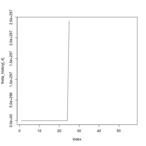

Definitely something not working there. Ok so now I’ll try it with feature scaling.

X[,2:3] <- feature_scale(X[,2:3])[[3]]
 
multi_lin_reg <- grad(
  alpha = 0.1,
  j = 1000,
  X = X,
  y = y,
  theta = theta
  ) %>% print

## $theta
##            [,1]
## [1,] 340412.660
## [2,] 110631.048
## [3,]  -6649.472
## 
## $cost
## [1] -6649.472
## 
## $iterations
## [1] 389

And to plot it:

plot(theta_history[,4],type="l")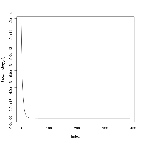

Great, convergence after 389 iterations. All seems well, but I want to compare this with a multiple linear regression the traditional way:

model <- lm(
  price ~ size + n_rooms,
  data = house_prices %>% mutate(n_rooms = as.integer(n_rooms))
  )
coef(model)

## (Intercept)        size     n_rooms 
##  89597.9095    139.2107  -8738.0191

The parameters don’t match, but this is because we have scaled the features. The output from the two models will be the same. Here I check by combining the two predictions into the house_prices dataframe, and comparing them with identical().

house_prices %<>%
  dplyr::mutate(
    
    # Vectorised method of theta transpose X
    
    vector_pred = (X %*% multi_lin_reg$theta),
    
    # Traditional statistical method of y = a + bx + cx
    
    pred = coef(model)[1] + (coef(model)[2] * size) + (coef(model)[3]*as.integer(n_rooms))
    )
 
identical(
  c(house_prices$vector_pred),
  c(house_prices$pred)
  )

## [1] FALSE

Ok not identical, how come?

(house_prices$pred - house_prices$vector_pred) %>% mean

## [1] 3.244767e-10

So they differ by a pretty small amount. Try the comparison more sensibly:

all.equal(
  c(house_prices$vector_pred),
  c(house_prices$pred)
  )

## [1] TRUE

And now let’s plot the actual data with predictions from the multiple regression.

house_prices %>%
  ggplot(
    aes(
      x = size,
      y = price,
      colour = n_rooms
      )
    ) +
  geom_point() +
  geom_point(
    aes(
      x = size,
      y = vector_pred
      ),
    shape = 2,
    )

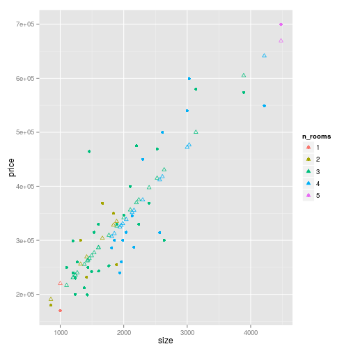
Pretty close to a single regression model, but you can see that there are slightly different slopes for each number of rooms.

Matt Upson

Recommended reading

Multivariate linear regression

Feature normalisation/scaling

Gradient descent

Matt Upson

Recommended reading

Multivariate linear regression

Feature normalisation/scaling

Gradient descent

You might also enjoy (View all posts)