
In my last post I compared vectorised logistic regression solved with an optimisation algorithm with a generalised linear model. I tested it out on a very simple dataset which could be classified using a linear boundary. In this post I’m following the next part of Andrew Ng’s Machine Learning course on coursera and implementing regularisation and feature mapping to allow me to map non-linear decision boundaries using logistic regression. And of course, I’m doing it in R, not Matlab or Octave.
As ever the full code to produce this page is available on github.
Visualising the data
First I plot the data…and it’s pretty clear that to create an accurate decision boundary will require some degree of polynomial features in order to account for its spherical nature.
library(dplyr)
library(magrittr)
library(ggplot2)
library(ucminf)
library(testthat)

ex2data2 <- "ex2data2.txt" %>%
  read.csv(header=FALSE) %>%
  set_colnames(c("test_1","test_2","passed"))

p <- ex2data2 %>%
  ggplot(
    aes(
      x = test_1,
      y = test_2
      )
    ) +
  geom_point(
    aes(
      shape = factor(passed),
      colour = factor(passed)
      )
    )+
  xlab("Microchip test 1")+
  ylab("Microchip test 2")

p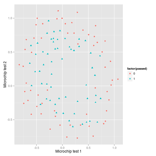
Feature mapping
In this example I’ll map the features into all polynomial terms of $x_1$ and $x_2$ up to the twelfth power giving a crazy amount of input features. Hence:
These polynomials can be calculated with the following code. In future I will update this to take more than two input features.
map_feature <- function(X1,X2,degree) {

  # There's probably a more mathematically succinct way of doing this...
  # Calculate the required ncol of the matrix

  counter = 0
  for (i in 1:degree){
    for (j in 0:i) {
      counter <- counter + 1
      }
    }

  out_matrix <- matrix(
    nrow = length(X1),
    ncol = counter
    )

  names_vec <- vector(
    length = counter
    )

  counter = 0
  for (i in 1:degree) {
    for (j in 0:i) {
      counter <- counter + 1
      out_matrix[,counter] <- ((X1^(i-j))*(X2^j))

      # Work out the names for the matrix

      names_vec[counter] <- paste("X1^",i-j,"*X2^",j,sep="")
      }
    }

  out_matrix <- cbind(1, out_matrix)
  colnames(out_matrix) <- c(1,names_vec)
  return(out_matrix)

  }
And to the list the 91 features:
degree <- 12

poly <- map_feature(
  ex2data2$test_1,
  ex2data2$test_2,
  degree
  )

poly %>% colnames
## [1] "1" "X1^1*X2^0" "X1^0*X2^1" "X1^2*X2^0" "X1^1*X2^1"
## [6] "X1^0*X2^2" "X1^3*X2^0" "X1^2*X2^1" "X1^1*X2^2" "X1^0*X2^3"
## [11] "X1^4*X2^0" "X1^3*X2^1" "X1^2*X2^2" "X1^1*X2^3" "X1^0*X2^4"
## [16] "X1^5*X2^0" "X1^4*X2^1" "X1^3*X2^2" "X1^2*X2^3" "X1^1*X2^4"
## [21] "X1^0*X2^5" "X1^6*X2^0" "X1^5*X2^1" "X1^4*X2^2" "X1^3*X2^3"
## [26] "X1^2*X2^4" "X1^1*X2^5" "X1^0*X2^6" "X1^7*X2^0" "X1^6*X2^1"
## [31] "X1^5*X2^2" "X1^4*X2^3" "X1^3*X2^4" "X1^2*X2^5" "X1^1*X2^6"
## [36] "X1^0*X2^7" "X1^8*X2^0" "X1^7*X2^1" "X1^6*X2^2" "X1^5*X2^3"
## [41] "X1^4*X2^4" "X1^3*X2^5" "X1^2*X2^6" "X1^1*X2^7" "X1^0*X2^8"
## [46] "X1^9*X2^0" "X1^8*X2^1" "X1^7*X2^2" "X1^6*X2^3" "X1^5*X2^4"
## [51] "X1^4*X2^5" "X1^3*X2^6" "X1^2*X2^7" "X1^1*X2^8" "X1^0*X2^9"
## [56] "X1^10*X2^0" "X1^9*X2^1" "X1^8*X2^2" "X1^7*X2^3" "X1^6*X2^4"
## [61] "X1^5*X2^5" "X1^4*X2^6" "X1^3*X2^7" "X1^2*X2^8" "X1^1*X2^9"
## [66] "X1^0*X2^10" "X1^11*X2^0" "X1^10*X2^1" "X1^9*X2^2" "X1^8*X2^3"
## [71] "X1^7*X2^4" "X1^6*X2^5" "X1^5*X2^6" "X1^4*X2^7" "X1^3*X2^8"
## [76] "X1^2*X2^9" "X1^1*X2^10" "X1^0*X2^11" "X1^12*X2^0" "X1^11*X2^1"
## [81] "X1^10*X2^2" "X1^9*X2^3" "X1^8*X2^4" "X1^7*X2^5" "X1^6*X2^6"
## [86] "X1^5*X2^7" "X1^4*X2^8" "X1^3*X2^9" "X1^2*X2^10" "X1^1*X2^11"
## [91] "X1^0*X2^12"Now run the linear regression I implemented in my previous post.
theta <- rep(0, ncol(poly))
y <- ex2data2$passed

ucminf_out <- ucminf(
  par = theta,
  fn = function(t) Jv(poly, y, t),
  gr = function(t) gRv(poly, y, t)
  )

ucminf_out$convergence
## [1] 4ucminf_out$message## [1] "Stopped by zero step from line search"So the optimisation algorithm converged successfully, and if I was to call ucminf_out$par, it would return our 91 parameters.
At this point it is probably worth defining some sort of measure of accuracy. A simple proportion error will suffice in this case.
err <- function(y,pred) {

  # Should really be implementing more unit tests throughout...

  test_that(
    "Prediction and actual are the same length",
    expect_equal(length(y),length(pred))
    )

  error <- 1/length(y) * sum((y - pred)^2)
  error <- round(error,2)
  return(error)

  }

# Proportion of data that is incorrectly classified

err(
  ex2data2$passed,
  h(ucminf_out$par,poly)
  )
## [1] 0.07So the present model accurately predicts 93% of the training data, but it is a pretty specific shape that is likely to be overfitted.
With just two original input features, we can quite easily plot the decision boundary. To do so I create a matrix $X$ of $m$ rows which corresponds to a grid of points for which we can then generate a prediction. We use the output $\theta$ derived from the model fit from the ex2data1 data. We then combine the predictions from the grid of points in a contour plot.
The function to create the boundary thus takes two inputs: a sequence of numbers xy delineating the limits of the plot. This works for situations where the ranges of the two features are similar, but would need to be adapted for features with different ranges (although it would probably be fine if feature scaling is used)
draw_boundary <- function(xy,theta,degree) {

  u <- rep(xy, times = length(xy))
  v <- rep(xy, each = length(xy))

  cbind(u,v,z = NA) %>%
    as.data.frame %>%
    tbl_df %>%
    dplyr::mutate(
      z = h(theta, map_feature(u,v,degree)) %>% round
      )
  }
Create the grid of predictions:
boundary <- draw_boundary(
  seq(-1.5, 1.5, length = 500),
  ucminf_out$par,
  degree
  )
And now for the decision boundary:
p + geom_contour(
  data = boundary,
  aes(
    x = u,
    y = v,
    z = z
    ),
  bins = 1
  )+
  coord_cartesian(
    xlim = c(-0.9,1.2),
    ylim = c(-0.9,1.2)
    )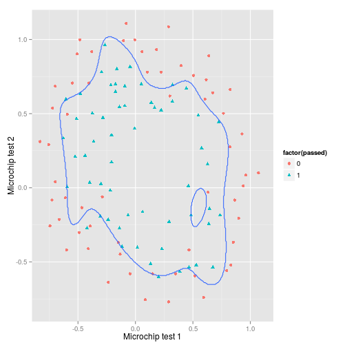
So this looks is capturing the positive values pretty well, but it could probably be improved especially in the top and bottom left where new cases are likely to be mis-classified.
Regularisation - cost function and gradient
To improve on the boundary above we can implement regularisation; this should reduce some of the overfitting seen in the last plot.
Andrew Ng gives us the regularised cost function as:
Note that the parameter $\theta_0$ is not regularised as this corresponds to the intercept.
Jv_reg <- function(X, y, theta, lambda) {

  m <- length(y)

  # Remove first value i.e. theta_0

  theta1 <- theta
  theta1[1] <- 0

  # Crossproduct is equivaelnt to theta[-1]^2

  reg <- (lambda/(2*m)) * crossprod(theta1,theta1)

  # Create regularisation term

  -(1/m) * crossprod(
    c(y, 1 - y),
    c(log(h(theta,X)), log(1 - h(theta,X)))
    ) + reg
  }
So let’s test this in comparison with the cost function that I defined in the previous post by setting the parameter $\lambda=0$, i.e. no regularisation.
all.equal(
  Jv(poly,y,theta),
  Jv_reg(poly,y,theta,0)
  )
## [1] TRUEGreat, the function passes this basic test. And the cost for all values of $\theta$ initialised to zero should be around $0.693$.
Jv_reg(poly,y,theta,0)## [,1]
## [1,] 0.6931472Now for the gradient function. As noted, we don’t regularise $\theta_0$, so we need a more complicated gradient function.
This can be implemented in vectorised fashion:
gRv_reg <- function(X,y,theta,lambda) {

  m <- length(y)

  reg <- (lambda/m) * theta
  error <- h(theta,X) - y
  delta <- crossprod(X,error) / m
  return(delta + reg)

  }
Now check that this gives the same result for the implementation without regularisation.
all.equal(
  gRv(poly,y,theta),
  gRv_reg(poly,y,theta,0)
  )
## [1] TRUESo far so good. Now I’ll try running regularised logistic regression for the polynomial example, but first I’ll wrap this into a function to save having to explicitly declare the parameters each time.
reg_lr <- function(X,y,theta,lambda) {

  ucminf_out <- ucminf(
    par = theta,
    fn = function(t) Jv_reg(X, y, t, lambda),
    gr = function(t) gRv_reg(X, y, t, lambda)
    )

  error <- err(
    y,
    h(ucminf_out$par,X)
    )

  return(
    list(
      theta = as.vector(ucminf_out$par),
      error = error
      )
    )

  }
So we can try this…
reg_lr_out <- reg_lr(
  X = poly,
  y = y,
  theta = theta,
  lambda = 1
  )

reg_lr_out
## $theta
## [1] 1.116795888 0.622142490 1.144381441 -1.760214959 -0.893246508
## [6] -1.210119424 0.259287641 -0.385567512 -0.378582876 -0.002113363
## [11] -1.262116648 -0.043880154 -0.627506940 -0.275767731 -0.954816713
## [16] -0.087929375 -0.206783162 -0.049800103 -0.279764342 -0.311163184
## [21] -0.209464841 -0.871690233 0.034226746 -0.295848645 0.015258988
## [26] -0.328545231 -0.153747438 -0.652765344 -0.212586493 -0.094079448
## [31] -0.042243458 -0.115997122 -0.034127849 -0.169591334 -0.213073869
## [36] -0.226615812 -0.618312146 0.040374942 -0.154958018 0.014430220
## [41] -0.130840414 0.013658394 -0.187500334 -0.105806945 -0.447151822
## [46] -0.238780084 -0.042082893 -0.036744504 -0.045987498 -0.018756874
## [51] -0.065146211 -0.013666503 -0.105994705 -0.146706656 -0.203949401
## [56] -0.451351638 0.032798742 -0.089688693 0.009685109 -0.057863261
## [61] 0.006237453 -0.068507640 0.012199324 -0.114344440 -0.080982886
## [66] -0.317099323 -0.226550777 -0.019006589 -0.029703171 -0.018856708
## [71] -0.012996508 -0.024383193 -0.006704414 -0.039146008 -0.002644283
## [76] -0.070252488 -0.105101718 -0.177581222 -0.338552450 0.023408734
## [81] -0.055668058 0.006591905 -0.028903065 0.002398368 -0.026917924
## [86] 0.004309776 -0.040090466 0.010951520 -0.074018464 -0.065810602
## [91] -0.236770557
##
## $error
## [1] 0.15And it seems to be working, but notice that with $\lambda=1$ the error has increased to 0.15. This doesn’t tell the whole story though as looking at the previous decision boundary suggests overfitting. So what about the decision boundary for $\lambda=1$?
boundary <- draw_boundary(
  seq(-1.5, 1.5, length = 500),
  reg_lr_out$theta,
  degree
  )

p + geom_contour(
  data = boundary,
  aes(
    x = u,
    y = v,
    z = z
    ),
  bins = 1
  )+
  coord_cartesian(
    xlim = c(-0.9,1.2),
    ylim = c(-0.9,1.2)
    )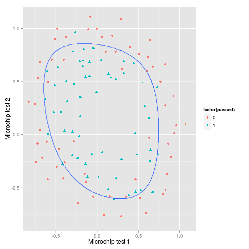
Regularisation has smoothed away much of the overfitting. We can’t tell how succesful this will be without evaluating the model on the a set, but we can also try a range of values for $\lambda$ and see what effect this has.
First compute the percentage errors for $\lambda={0,0.0001,0.001,0.01,0.1,1}$.
lambda <- c(0,0.0001,0.001,0.01,0.1,1)

reg_error <- matrix(ncol = 2, nrow = length(lambda))
for (i in 1:length(lambda)) {

  reg_error[i,1] <- lambda[i]
  reg_error[i,2] <- reg_lr(
    X = poly,
    y = y,
    theta = theta,
    lambda = lambda[i]
    ) %$% error
  }

reg_error %>% set_colnames(c("i","error"))
## i error
## [1,] 0e+00 0.07
## [2,] 1e-04 0.08
## [3,] 1e-03 0.09
## [4,] 1e-02 0.10
## [5,] 1e-01 0.11
## [6,] 1e+00 0.15So it looks like increasing $\lambda$ is reducing the accuracy of the model on the training set. But again, this isn’t the whole story. What about the decision boundaries?
# Generate boundaries for a number of lambdas

out_mat <- matrix(nrow = 500, ncol = length(lambda))
colnames(out_mat) <- paste(lambda, sep = "")
out_mat <- cbind(boundary[,1:2],out_mat) %>% as.matrix

# Add two 0s to the beginning of the vector to make life easier in the for loop
# when referencing lambda

lambda <- c(0,0,lambda)

for (i in 3:ncol(out_mat)) {

  out <- draw_boundary(
    seq(-1.5, 1.5, length = 500),
    reg_lr(
      X = poly,
      y = y,
      theta = theta,
      lambda = lambda[i]
      )$theta,
    degree
    ) %$% z %>% as.vector

  out_mat[,i] <- out

  }
Now use tidyr::gather to turn this wide data into long data so it can be passed to ggplot2::facet_wrap.
out_mat %>%
  data.frame %>%
  tidyr::gather(
    key,value,3:ncol(out_mat)
    ) %>%
  tbl_df  %>%
  ggplot(
    aes(
      x = u,
      y = v
      )
    ) +
  geom_contour(
    aes(
      z = value
      ),
    bins = 1
    ) +
  facet_wrap(
    ~key,
    ncol = 2
    ) +
  geom_point(
    data = ex2data2,
    aes(
      x = test_1,
      y = test_2,
      colour = factor(passed),
      shape = factor(passed)
      )
    ) +
  xlab("Microchip test 1") +
  ylab("Microchip test 2") +
  coord_cartesian(
    xlim = c(-0.9,1.2),
    ylim = c(-0.9,1.2)
    )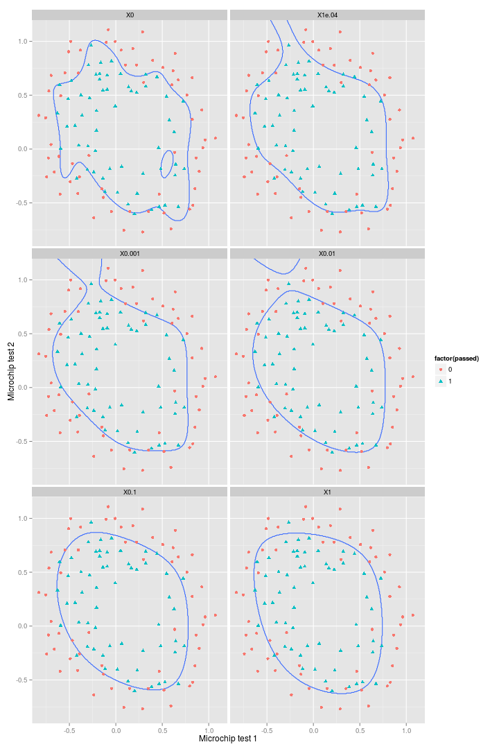
So it’s clear that increasing $\lambda$ leads to progressively greater smoothing of the decision boundary. And despite decreasing accuracy on the training set, these regularised decision boundaries would certainly perform better against a test set.
sessionInfo()## R version 3.1.3 (2015-03-09)
## Platform: x86_64-pc-linux-gnu (64-bit)
## Running under: Ubuntu 14.04.2 LTS
##
## locale:
## [1] LC_CTYPE=en_GB.UTF-8 LC_NUMERIC=C
## [3] LC_TIME=en_GB.UTF-8 LC_COLLATE=en_GB.UTF-8
## [5] LC_MONETARY=en_GB.UTF-8 LC_MESSAGES=en_GB.UTF-8
## [7] LC_PAPER=en_GB.UTF-8 LC_NAME=C
## [9] LC_ADDRESS=C LC_TELEPHONE=C
## [11] LC_MEASUREMENT=en_GB.UTF-8 LC_IDENTIFICATION=C
##
## attached base packages:
## [1] methods stats graphics grDevices utils datasets base
##
## other attached packages:
## [1] ucminf_1.1-3 ggplot2_1.0.0 magrittr_1.5 dplyr_0.4.1
## [5] testthat_0.8.1 knitr_1.9
##
## loaded via a namespace (and not attached):
## [1] assertthat_0.1 colorspace_1.2-5 DBI_0.3.1 digest_0.6.4
## [5] evaluate_0.5.5 formatR_1.0 grid_3.1.3 gtable_0.1.2
## [9] labeling_0.3 lazyeval_0.1.10 MASS_7.3-39 munsell_0.4.2
## [13] parallel_3.1.3 plyr_1.8.1 proto_0.3-10 Rcpp_0.11.5
## [17] reshape2_1.4.1 scales_0.2.4 stringr_0.6.2 tcltk_3.1.3
## [21] tidyr_0.2.0 tools_3.1.3