
In this post I reproduce an example similar to an exercise I did for the coursera MOOC course in machine learning written by Andrew Ng. I’m compelting the course musing R, not the requisite matlab. In the next couple of posts I’m going to complete the equivalent of exercise 5.
The exercise was about creating a vectorised implementation of regularised linear regression, and using this to test some theory relating to the diagnosis of bias (underfitting) and variance (overfitting). I will use a different, but similar dataset to avoid publishing the solutions here.
What is regularisation all about?
Regularisation helps us to deal with the problem of overfitting by reducing the weight given to a particular feature $x$. This allows us to retain more features while not giving undue weight to one in particular. Regularisation is mediated by a parameter $\lambda$, as can be seen in the cost function:
The first term is essentially the mean-squared-error term, whilst the additive term multiplies the sum of the square of the parameters ($\theta$) by $\lambda$ over $2m$, where $m$ is the number of training examples. Since the objective is to minimise $J(\theta)$ ($\underset{\theta}{\text{min}}J(\theta)$) using a large $\lambda$ will require small values of $\theta_j$ in order to acheive a minima.
Getting some data
In this example I’m using data from the well worn mtcars dataset which is included in the datasets package, instead of the data given in the course. For the first example presented here, I limit myself to just the first five columns of this dataset, which are: mpg, cyl, disp, and hp, or: miles per gallon, number of cylinders, displacement ($\text{in}^2$), and gross horsepower (run ?mtcars for a data description). In this example, I want to predict mpg using cyl, disp, and hp as features.
Plotting each individually gives us a sense that they all have pretty correlations with mpg, but it’s also obvious that the features are correlated: e.g. disp and hp.
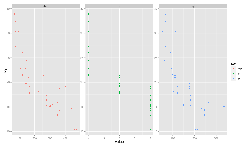
We can also see that the range of values that the features take vary quite a lot. Whilst cyl $\leq{8}$, disp tends to measured in the hundreds of $\text{in}^2$.
mtcars[1:4] %>% summary## mpg cyl disp hp
## Min. :10.40 Min. :4.000 Min. : 71.1 Min. : 52.0
## 1st Qu.:15.43 1st Qu.:4.000 1st Qu.:120.8 1st Qu.: 96.5
## Median :19.20 Median :6.000 Median :196.3 Median :123.0
## Mean :20.09 Mean :6.188 Mean :230.7 Mean :146.7
## 3rd Qu.:22.80 3rd Qu.:8.000 3rd Qu.:326.0 3rd Qu.:180.0
## Max. :33.90 Max. :8.000 Max. :472.0 Max. :335.0There are 32 rows in the data set, and for this example I will make a 60/20/20 split on the dataset for train/cross-validate/test, giving 19 rows in the test set, and 6 and 7 in the cross-validation and test sets respectively.
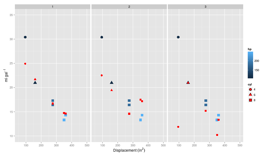
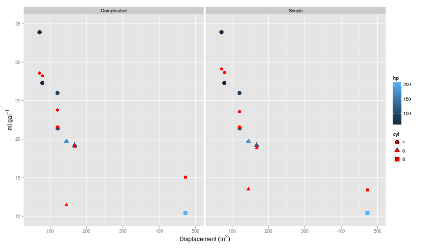
At this point is has already become a little difficult to display all the features on a simple two dimensional plot, so I’ll use a combination of colour and shape.
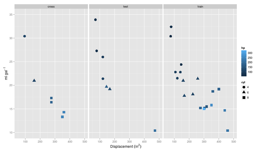
So each split of the data has retained some semblance of the curvature present in the training set.
Regularised linear regression
To run the linear regression, I’ll build on the vectorised linear regression implementation I implemented here, but this time including a regularisation term.
A vectorised implementation of the cost function is given below. Note I’ve used tcrossprod(theta, X) as this function was about 1.5 times quicker than the equivalent X %*% theta in my tests, and both return the result of $\theta^TX$.
The cost function is not applied to $\theta_0$ as this relates to the intercept parameter.
J <- function(X, y, theta, lambda) {

  m <- length(y)

  theta1 <- theta

  # Ensure that regularisation is not operating on \theta_0

  theta1[1] <- 0

  error <- tcrossprod(theta,X)
  error <- as.vector(error) - y
  error1 <- crossprod(error,error)

  reg <- (lambda/(2*m)) * crossprod(theta1, theta1)

  cost <- (1/(2 * m)) * error1 + reg

  return(cost)

  }
The gradient function is given below, and is the same as that given in my previous post on regularised logistic regression Note that once again the regularisation term excludes $\theta_0$.
gR <- function(X, y, theta, lambda) {

  theta1 <- theta
  theta1[1] <- 0

  m <- length(y)

  error <- tcrossprod(theta,X)
  error <- as.vector(error) - y
  error <- (1/m) * crossprod(error,X)

  reg <- (lambda/(m)) * theta1

  delta <- error + reg

  return(delta)

  }
Optimisation algorithm
As an optimisation algorithm, I’m use the optim function which ships with the stats package in vanilla R. Previously I used the ucminf function, and these two take the same arguments, so switching out the algorithms in the code is very simple. As default I have stuck to the BFGS method, and to $\lambda=0$, i.e. no regularisation.
I’ve also just included the parameters as they are, so any solutions are going to be strictly linear, and therefore many not be a very good fit.
X <- cbind(1,train$cyl,train$disp,train$hp)
y <- train$mpg

theta <- rep(1, ncol(X))
lambda <- 0

ucminf_out <- optim(
  par = theta,
  fn = function(t) J(X, y, t, lambda),
  gr = function(t) gR(X, y, t, lambda),
  method = "BFGS"
  )
So far so good, this seems to work:
## $par
## [1] 30.25511907 -2.38150554 -0.01374584 -0.01450777
##
## $value
## [1] 3.948106
##
## $counts
## function gradient
##       71       28
##
## $convergence
## [1] 0
##
## $message
## NULL
The output from optim differs slightly from ucminf; here a convergence of $0$ indicates success, and includes the number of times the cost function and gradient functions were called ($counts). The output also gives the final cost ($value) associated with the parameters ($par). For the most part, we are only interested in the parameters themselves, which we can plug into ggplot to overlay the model onto the training set.
Let’s compare the training data with the new predictions from the model trained on that data.
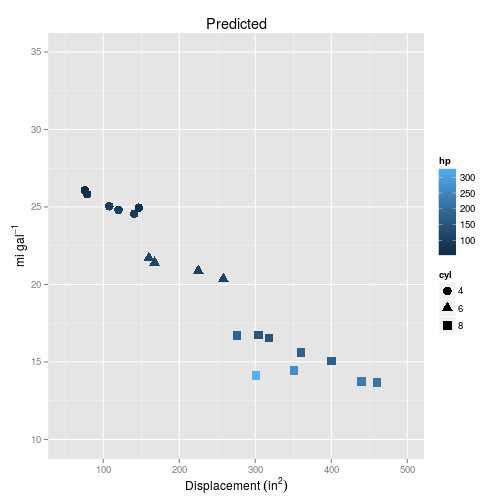
So based on these plots, it should be pretty clear that the simple multiple regression is too simple to represent the curvature we can see in the data.
We can calculate the error related to this model using the sum of the squared differences between the expected and the observed:
J_train <- function(predicted, actual) {

  m <- length(y)

  error <- predicted - actual
  error <- crossprod(error, error)

  return(
      (1/m) * error
  )

}
Applying this function to the existing model gives a training error of $7.90$.
Polynomials
So one way of taking account of the curvature in the data is to add features to the data, for example polynomials of the input matrix $X$.
Part of the coursera exercise is to create a function to produce polynomials of different features (explanatory variables), but R has a built in polynomial function in the stats package: poly which is $50\%$ faster than the equivalent function that I wrote, so I’ll stick to this.
Since we have three features, using three degrees of polynomial will result in $19$ features in total on $19$ training examples. One feature for every training example sounds like a lot, and will almost certainly lead to over-fitting, so it should be a good way of demonstrating regularisation.
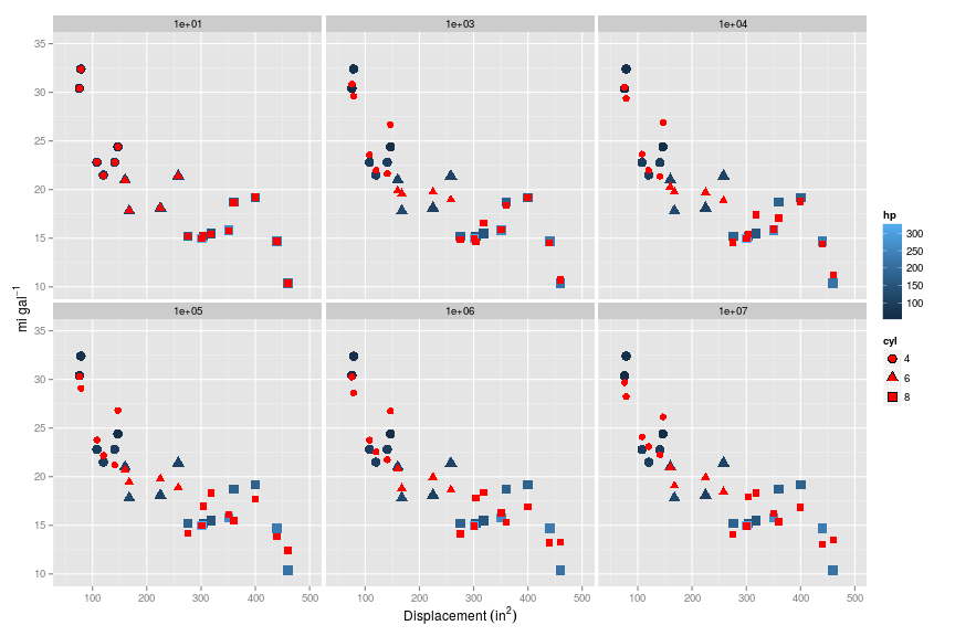
The plot below shows the results from models trained on first (i.e. no polynomial) to third order polynomials on the training set (red points are the predicted values).
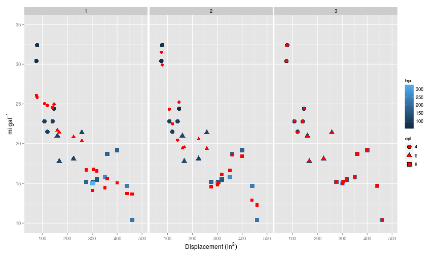
So as before, the first model has made a linear prediction, whilst including second and third order polynomials takes into account the curvature at least in the disp $\times$ mpg relationship. Note that the model including the third order polynomials has achieved close to 100% accuracy, because there is one feature per training example.
Comparing the model errors confirms this assessment. The training error for the third order polynomial is almost zero, whilst the second order polynomial provides an improvement over the simple linear model.
## Source: local data frame [3 x 2]
##
##   degree       error
## 1      1 7.896211930
## 2      2 2.197951280
## 3      3 0.001151986
Cross validation
So what happens when we apply these models onto the cross-validation dataset. If intuition holds true, the second order model should provide the best fit, whilst the third order model should show signs of having been overfit on the training data.
So as predicted, it looks like the third order polynomial model is the worst, as is shown when calculating the error:
## Source: local data frame [3 x 2]
##
##   degree     error
## 1      1  1.740409
## 2      2  5.333678
## 3      3 18.912658
Interestingly, the simplest model, without any curvature performs the best on this cross validation set, when no regularisation is specified. This may not be surprising given that it is such a small subset of the data.
Regularisation
So what happens when we apply regularisation?. I’ll start with the extreme example: applying regularisation to the the over-fitted model with third order polynomials. Since I am trying here to reduce the impact that particular features have on the model, intuitively this should mean that I will need a relatively large $\lambda$.
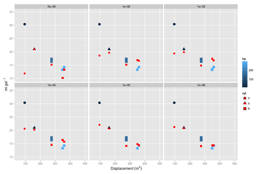
Let’s start with $\lambda = {10,100,1000,10000,100000,1000000}$, and look what happens to the prediction of mpg from the training set. As $\lambda$ increases, the prediction becomes increasingly more generalised, and fits the training set less perfectly…
And when applied to the cross validation set, increasing $\lambda$ improves the fit of predictions to the cross validation set.
And what about the error? Plotting the training error versus cross-validation error will give us an impression of what effect the regularisation parameter is having.
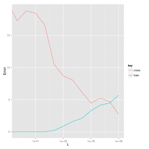
So it looks like a value of around $10^7$ will minimise both the training and cross-validation error. This is a pretty large $\lambda$ - but this may not be surprising given that a three order polynomial generates $19$ features for just $19$ training examples, i.e $m=k$.
I’m interested to know what would have happened if I had chosen to run with the second order polynomial model. Using the same choices for $\lambda$ is not appropriate for this model, as there are only $9$ features, so this time I have chosen a smaller range of $\lambda$, but retained $10^7$ just to see what would happen.

So in this case, setting $\lambda = 10^7$ is a step too far, and results in a model that is too simple, and loses the curvature evident in the data.
And the error?

As predicted, $\lambda$ needs to be set much lower, between $10$ and $100$ to obtain the best solution for the training and cross-validation set. Interestingly the cross-validation error continues to drop until about $\lambda=10000$ which coincides with the model failing to predict curvature in the data as above.
Wrapping up
So the final question remains. How will these two models perform against each other: a more complicated model with a very high $\lambda$, or a simpler model with a lower $\lambda$?
There is almost no difference between the performance of the models on the test set; both do a reasonable job; the third order polynomial model gives an error of 1.03, which is very similar to the error given by the simpler model 1.00.
Of course, I should point out that something is probably going wrong if the number of features ($k$) equals the number of training examples ($m$); it’s as overfitted as a model can get; but it demonstrates the power of regularisation, and it is heartening to see that a simpler model can perform just as well.
sessionInfo()## R version 3.2.0 (2015-04-16)
## Platform: x86_64-unknown-linux-gnu (64-bit)
## Running under: Ubuntu 14.04.2 LTS
##
## locale:
## [1] LC_CTYPE=en_GB.UTF-8 LC_NUMERIC=C
## [3] LC_TIME=en_GB.UTF-8 LC_COLLATE=en_GB.UTF-8
## [5] LC_MONETARY=en_GB.UTF-8 LC_MESSAGES=en_GB.UTF-8
## [7] LC_PAPER=en_GB.UTF-8 LC_NAME=C
## [9] LC_ADDRESS=C LC_TELEPHONE=C
## [11] LC_MEASUREMENT=en_GB.UTF-8 LC_IDENTIFICATION=C
##
## attached base packages:
## [1] methods stats graphics grDevices utils datasets base
##
## other attached packages:
## [1] RColorBrewer_1.1-2 tidyr_0.2.0 ggplot2_1.0.1
## [4] ucminf_1.1-3 boot_1.3-16 magrittr_1.5
## [7] dplyr_0.4.1 testthat_0.9.1 knitr_1.10
##
## loaded via a namespace (and not attached):
## [1] Rcpp_0.11.5 MASS_7.3-40 munsell_0.4.2 colorspace_1.2-6
## [5] stringr_1.0.0 plyr_1.8.2 tools_3.2.0 parallel_3.2.0
## [9] grid_3.2.0 gtable_0.1.2 DBI_0.3.1 lazyeval_0.1.10
## [13] assertthat_0.1 digest_0.6.8 reshape2_1.4.1 formatR_1.2
## [17] evaluate_0.7 labeling_0.3 stringi_0.4-1 scales_0.2.4
## [21] proto_0.3-10